*Heading
** Job name: Job-1 Model name: Model-1
** Generated by: Abaqus/CAE 2018
*Preprint, echo=NO, model=NO, history=NO, contact=NO
**
** PARTS
**
*Part, name=Part-1
*Node
      1,         -0.5,         -0.5
      2, -0.400000006,         -0.5
      3, -0.300000012,         -0.5
      4, -0.200000003,         -0.5
      5, -0.100000001,         -0.5
      6,           0.,         -0.5
      7,  0.100000001,         -0.5
      8,  0.200000003,         -0.5
      9,  0.300000012,         -0.5
     10,  0.400000006,         -0.5
     11,          0.5,         -0.5
     12,         -0.5, -0.400000006
     13, -0.400000006, -0.400000006
     14, -0.300000012, -0.400000006
     15, -0.200000003, -0.400000006
     16, -0.100000001, -0.400000006
     17,           0., -0.400000006
     18,  0.100000001, -0.400000006
     19,  0.200000003, -0.400000006
     20,  0.300000012, -0.400000006
     21,  0.400000006, -0.400000006
     22,          0.5, -0.400000006
     23,         -0.5, -0.300000012
     24, -0.400000006, -0.300000012
     25, -0.300000012, -0.300000012
     26, -0.200000003, -0.300000012
     27, -0.100000001, -0.300000012
     28,           0., -0.300000012
     29,  0.100000001, -0.300000012
     30,  0.200000003, -0.300000012
     31,  0.300000012, -0.300000012
     32,  0.400000006, -0.300000012
     33,          0.5, -0.300000012
     34,         -0.5, -0.200000003
     35, -0.400000006, -0.200000003
     36, -0.300000012, -0.200000003
     37, -0.200000003, -0.200000003
     38, -0.100000001, -0.200000003
     39,           0., -0.200000003
     40,  0.100000001, -0.200000003
     41,  0.200000003, -0.200000003
     42,  0.300000012, -0.200000003
     43,  0.400000006, -0.200000003
     44,          0.5, -0.200000003
     45,         -0.5, -0.100000001
     46, -0.400000006, -0.100000001
     47, -0.300000012, -0.100000001
     48, -0.200000003, -0.100000001
     49, -0.100000001, -0.100000001
     50,           0., -0.100000001
     51,  0.100000001, -0.100000001
     52,  0.200000003, -0.100000001
     53,  0.300000012, -0.100000001
     54,  0.400000006, -0.100000001
     55,          0.5, -0.100000001
     56,         -0.5,           0.
     57, -0.400000006,           0.
     58, -0.300000012,           0.
     59, -0.200000003,           0.
     60, -0.100000001,           0.
     61,           0.,           0.
     62,  0.100000001,           0.
     63,  0.200000003,           0.
     64,  0.300000012,           0.
     65,  0.400000006,           0.
     66,          0.5,           0.
     67,         -0.5,  0.100000001
     68, -0.400000006,  0.100000001
     69, -0.300000012,  0.100000001
     70, -0.200000003,  0.100000001
     71, -0.100000001,  0.100000001
     72,           0.,  0.100000001
     73,  0.100000001,  0.100000001
     74,  0.200000003,  0.100000001
     75,  0.300000012,  0.100000001
     76,  0.400000006,  0.100000001
     77,          0.5,  0.100000001
     78,         -0.5,  0.200000003
     79, -0.400000006,  0.200000003
     80, -0.300000012,  0.200000003
     81, -0.200000003,  0.200000003
     82, -0.100000001,  0.200000003
     83,           0.,  0.200000003
     84,  0.100000001,  0.200000003
     85,  0.200000003,  0.200000003
     86,  0.300000012,  0.200000003
     87,  0.400000006,  0.200000003
     88,          0.5,  0.200000003
     89,         -0.5,  0.300000012
     90, -0.400000006,  0.300000012
     91, -0.300000012,  0.300000012
     92, -0.200000003,  0.300000012
     93, -0.100000001,  0.300000012
     94,           0.,  0.300000012
     95,  0.100000001,  0.300000012
     96,  0.200000003,  0.300000012
     97,  0.300000012,  0.300000012
     98,  0.400000006,  0.300000012
     99,          0.5,  0.300000012
    100,         -0.5,  0.400000006
    101, -0.400000006,  0.400000006
    102, -0.300000012,  0.400000006
    103, -0.200000003,  0.400000006
    104, -0.100000001,  0.400000006
    105,           0.,  0.400000006
    106,  0.100000001,  0.400000006
    107,  0.200000003,  0.400000006
    108,  0.300000012,  0.400000006
    109,  0.400000006,  0.400000006
    110,          0.5,  0.400000006
    111,         -0.5,          0.5
    112, -0.400000006,          0.5
    113, -0.300000012,          0.5
    114, -0.200000003,          0.5
    115, -0.100000001,          0.5
    116,           0.,          0.5
    117,  0.100000001,          0.5
    118,  0.200000003,          0.5
    119,  0.300000012,          0.5
    120,  0.400000006,          0.5
    121,          0.5,          0.5
    122, -0.449999988,         -0.5
    123, -0.400000006, -0.449999988
    124, -0.449999988, -0.400000006
    125,         -0.5, -0.449999988
    126, -0.350000024,         -0.5
    127, -0.300000012, -0.449999988
    128, -0.350000024, -0.400000006
    129,        -0.25,         -0.5
    130, -0.200000003, -0.449999988
    131,        -0.25, -0.400000006
    132, -0.150000006,         -0.5
    133, -0.100000001, -0.449999988
    134, -0.150000006, -0.400000006
    135, -0.0500000007,         -0.5
    136,           0., -0.449999988
    137, -0.0500000007, -0.400000006
    138, 0.0500000007,         -0.5
    139,  0.100000001, -0.449999988
    140, 0.0500000007, -0.400000006
    141,  0.150000006,         -0.5
    142,  0.200000003, -0.449999988
    143,  0.150000006, -0.400000006
    144,         0.25,         -0.5
    145,  0.300000012, -0.449999988
    146,         0.25, -0.400000006
    147,  0.350000024,         -0.5
    148,  0.400000006, -0.449999988
    149,  0.350000024, -0.400000006
    150,  0.449999988,         -0.5
    151,          0.5, -0.449999988
    152,  0.449999988, -0.400000006
    153, -0.400000006, -0.350000024
    154, -0.449999988, -0.300000012
    155,         -0.5, -0.350000024
    156, -0.300000012, -0.350000024
    157, -0.350000024, -0.300000012
    158, -0.200000003, -0.350000024
    159,        -0.25, -0.300000012
    160, -0.100000001, -0.350000024
    161, -0.150000006, -0.300000012
    162,           0., -0.350000024
    163, -0.0500000007, -0.300000012
    164,  0.100000001, -0.350000024
    165, 0.0500000007, -0.300000012
    166,  0.200000003, -0.350000024
    167,  0.150000006, -0.300000012
    168,  0.300000012, -0.350000024
    169,         0.25, -0.300000012
    170,  0.400000006, -0.350000024
    171,  0.350000024, -0.300000012
    172,          0.5, -0.350000024
    173,  0.449999988, -0.300000012
    174, -0.400000006,        -0.25
    175, -0.449999988, -0.200000003
    176,         -0.5,        -0.25
    177, -0.300000012,        -0.25
    178, -0.350000024, -0.200000003
    179, -0.200000003,        -0.25
    180,        -0.25, -0.200000003
    181, -0.100000001,        -0.25
    182, -0.150000006, -0.200000003
    183,           0.,        -0.25
    184, -0.0500000007, -0.200000003
    185,  0.100000001,        -0.25
    186, 0.0500000007, -0.200000003
    187,  0.200000003,        -0.25
    188,  0.150000006, -0.200000003
    189,  0.300000012,        -0.25
    190,         0.25, -0.200000003
    191,  0.400000006,        -0.25
    192,  0.350000024, -0.200000003
    193,          0.5,        -0.25
    194,  0.449999988, -0.200000003
    195, -0.400000006, -0.150000006
    196, -0.449999988, -0.100000001
    197,         -0.5, -0.150000006
    198, -0.300000012, -0.150000006
    199, -0.350000024, -0.100000001
    200, -0.200000003, -0.150000006
    201,        -0.25, -0.100000001
    202, -0.100000001, -0.150000006
    203, -0.150000006, -0.100000001
    204,           0., -0.150000006
    205, -0.0500000007, -0.100000001
    206,  0.100000001, -0.150000006
    207, 0.0500000007, -0.100000001
    208,  0.200000003, -0.150000006
    209,  0.150000006, -0.100000001
    210,  0.300000012, -0.150000006
    211,         0.25, -0.100000001
    212,  0.400000006, -0.150000006
    213,  0.350000024, -0.100000001
    214,          0.5, -0.150000006
    215,  0.449999988, -0.100000001
    216, -0.400000006, -0.0500000007
    217, -0.449999988,           0.
    218,         -0.5, -0.0500000007
    219, -0.300000012, -0.0500000007
    220, -0.350000024,           0.
    221, -0.200000003, -0.0500000007
    222,        -0.25,           0.
    223, -0.100000001, -0.0500000007
    224, -0.150000006,           0.
    225,           0., -0.0500000007
    226, -0.0500000007,           0.
    227,  0.100000001, -0.0500000007
    228, 0.0500000007,           0.
    229,  0.200000003, -0.0500000007
    230,  0.150000006,           0.
    231,  0.300000012, -0.0500000007
    232,         0.25,           0.
    233,  0.400000006, -0.0500000007
    234,  0.350000024,           0.
    235,          0.5, -0.0500000007
    236,  0.449999988,           0.
    237, -0.400000006, 0.0500000007
    238, -0.449999988,  0.100000001
    239,         -0.5, 0.0500000007
    240, -0.300000012, 0.0500000007
    241, -0.350000024,  0.100000001
    242, -0.200000003, 0.0500000007
    243,        -0.25,  0.100000001
    244, -0.100000001, 0.0500000007
    245, -0.150000006,  0.100000001
    246,           0., 0.0500000007
    247, -0.0500000007,  0.100000001
    248,  0.100000001, 0.0500000007
    249, 0.0500000007,  0.100000001
    250,  0.200000003, 0.0500000007
    251,  0.150000006,  0.100000001
    252,  0.300000012, 0.0500000007
    253,         0.25,  0.100000001
    254,  0.400000006, 0.0500000007
    255,  0.350000024,  0.100000001
    256,          0.5, 0.0500000007
    257,  0.449999988,  0.100000001
    258, -0.400000006,  0.150000006
    259, -0.449999988,  0.200000003
    260,         -0.5,  0.150000006
    261, -0.300000012,  0.150000006
    262, -0.350000024,  0.200000003
    263, -0.200000003,  0.150000006
    264,        -0.25,  0.200000003
    265, -0.100000001,  0.150000006
    266, -0.150000006,  0.200000003
    267,           0.,  0.150000006
    268, -0.0500000007,  0.200000003
    269,  0.100000001,  0.150000006
    270, 0.0500000007,  0.200000003
    271,  0.200000003,  0.150000006
    272,  0.150000006,  0.200000003
    273,  0.300000012,  0.150000006
    274,         0.25,  0.200000003
    275,  0.400000006,  0.150000006
    276,  0.350000024,  0.200000003
    277,          0.5,  0.150000006
    278,  0.449999988,  0.200000003
    279, -0.400000006,         0.25
    280, -0.449999988,  0.300000012
    281,         -0.5,         0.25
    282, -0.300000012,         0.25
    283, -0.350000024,  0.300000012
    284, -0.200000003,         0.25
    285,        -0.25,  0.300000012
    286, -0.100000001,         0.25
    287, -0.150000006,  0.300000012
    288,           0.,         0.25
    289, -0.0500000007,  0.300000012
    290,  0.100000001,         0.25
    291, 0.0500000007,  0.300000012
    292,  0.200000003,         0.25
    293,  0.150000006,  0.300000012
    294,  0.300000012,         0.25
    295,         0.25,  0.300000012
    296,  0.400000006,         0.25
    297,  0.350000024,  0.300000012
    298,          0.5,         0.25
    299,  0.449999988,  0.300000012
    300, -0.400000006,  0.350000024
    301, -0.449999988,  0.400000006
    302,         -0.5,  0.350000024
    303, -0.300000012,  0.350000024
    304, -0.350000024,  0.400000006
    305, -0.200000003,  0.350000024
    306,        -0.25,  0.400000006
    307, -0.100000001,  0.350000024
    308, -0.150000006,  0.400000006
    309,           0.,  0.350000024
    310, -0.0500000007,  0.400000006
    311,  0.100000001,  0.350000024
    312, 0.0500000007,  0.400000006
    313,  0.200000003,  0.350000024
    314,  0.150000006,  0.400000006
    315,  0.300000012,  0.350000024
    316,         0.25,  0.400000006
    317,  0.400000006,  0.350000024
    318,  0.350000024,  0.400000006
    319,          0.5,  0.350000024
    320,  0.449999988,  0.400000006
    321, -0.400000006,  0.449999988
    322, -0.449999988,          0.5
    323,         -0.5,  0.449999988
    324, -0.300000012,  0.449999988
    325, -0.350000024,          0.5
    326, -0.200000003,  0.449999988
    327,        -0.25,          0.5
    328, -0.100000001,  0.449999988
    329, -0.150000006,          0.5
    330,           0.,  0.449999988
    331, -0.0500000007,          0.5
    332,  0.100000001,  0.449999988
    333, 0.0500000007,          0.5
    334,  0.200000003,  0.449999988
    335,  0.150000006,          0.5
    336,  0.300000012,  0.449999988
    337,         0.25,          0.5
    338,  0.400000006,  0.449999988
    339,  0.350000024,          0.5
    340,          0.5,  0.449999988
    341,  0.449999988,          0.5
*Element, type=CPE8R
  1,   1,   2,  13,  12, 122, 123, 124, 125
  2,   2,   3,  14,  13, 126, 127, 128, 123
  3,   3,   4,  15,  14, 129, 130, 131, 127
  4,   4,   5,  16,  15, 132, 133, 134, 130
  5,   5,   6,  17,  16, 135, 136, 137, 133
  6,   6,   7,  18,  17, 138, 139, 140, 136
  7,   7,   8,  19,  18, 141, 142, 143, 139
  8,   8,   9,  20,  19, 144, 145, 146, 142
  9,   9,  10,  21,  20, 147, 148, 149, 145
 10,  10,  11,  22,  21, 150, 151, 152, 148
 11,  12,  13,  24,  23, 124, 153, 154, 155
 12,  13,  14,  25,  24, 128, 156, 157, 153
 13,  14,  15,  26,  25, 131, 158, 159, 156
 14,  15,  16,  27,  26, 134, 160, 161, 158
 15,  16,  17,  28,  27, 137, 162, 163, 160
 16,  17,  18,  29,  28, 140, 164, 165, 162
 17,  18,  19,  30,  29, 143, 166, 167, 164
 18,  19,  20,  31,  30, 146, 168, 169, 166
 19,  20,  21,  32,  31, 149, 170, 171, 168
 20,  21,  22,  33,  32, 152, 172, 173, 170
 21,  23,  24,  35,  34, 154, 174, 175, 176
 22,  24,  25,  36,  35, 157, 177, 178, 174
 23,  25,  26,  37,  36, 159, 179, 180, 177
 24,  26,  27,  38,  37, 161, 181, 182, 179
 25,  27,  28,  39,  38, 163, 183, 184, 181
 26,  28,  29,  40,  39, 165, 185, 186, 183
 27,  29,  30,  41,  40, 167, 187, 188, 185
 28,  30,  31,  42,  41, 169, 189, 190, 187
 29,  31,  32,  43,  42, 171, 191, 192, 189
 30,  32,  33,  44,  43, 173, 193, 194, 191
 31,  34,  35,  46,  45, 175, 195, 196, 197
 32,  35,  36,  47,  46, 178, 198, 199, 195
 33,  36,  37,  48,  47, 180, 200, 201, 198
 34,  37,  38,  49,  48, 182, 202, 203, 200
 35,  38,  39,  50,  49, 184, 204, 205, 202
 36,  39,  40,  51,  50, 186, 206, 207, 204
 37,  40,  41,  52,  51, 188, 208, 209, 206
 38,  41,  42,  53,  52, 190, 210, 211, 208
 39,  42,  43,  54,  53, 192, 212, 213, 210
 40,  43,  44,  55,  54, 194, 214, 215, 212
 41,  45,  46,  57,  56, 196, 216, 217, 218
 42,  46,  47,  58,  57, 199, 219, 220, 216
 43,  47,  48,  59,  58, 201, 221, 222, 219
 44,  48,  49,  60,  59, 203, 223, 224, 221
 45,  49,  50,  61,  60, 205, 225, 226, 223
 46,  50,  51,  62,  61, 207, 227, 228, 225
 47,  51,  52,  63,  62, 209, 229, 230, 227
 48,  52,  53,  64,  63, 211, 231, 232, 229
 49,  53,  54,  65,  64, 213, 233, 234, 231
 50,  54,  55,  66,  65, 215, 235, 236, 233
 51,  56,  57,  68,  67, 217, 237, 238, 239
 52,  57,  58,  69,  68, 220, 240, 241, 237
 53,  58,  59,  70,  69, 222, 242, 243, 240
 54,  59,  60,  71,  70, 224, 244, 245, 242
 55,  60,  61,  72,  71, 226, 246, 247, 244
 56,  61,  62,  73,  72, 228, 248, 249, 246
 57,  62,  63,  74,  73, 230, 250, 251, 248
 58,  63,  64,  75,  74, 232, 252, 253, 250
 59,  64,  65,  76,  75, 234, 254, 255, 252
 60,  65,  66,  77,  76, 236, 256, 257, 254
 61,  67,  68,  79,  78, 238, 258, 259, 260
 62,  68,  69,  80,  79, 241, 261, 262, 258
 63,  69,  70,  81,  80, 243, 263, 264, 261
 64,  70,  71,  82,  81, 245, 265, 266, 263
 65,  71,  72,  83,  82, 247, 267, 268, 265
 66,  72,  73,  84,  83, 249, 269, 270, 267
 67,  73,  74,  85,  84, 251, 271, 272, 269
 68,  74,  75,  86,  85, 253, 273, 274, 271
 69,  75,  76,  87,  86, 255, 275, 276, 273
 70,  76,  77,  88,  87, 257, 277, 278, 275
 71,  78,  79,  90,  89, 259, 279, 280, 281
 72,  79,  80,  91,  90, 262, 282, 283, 279
 73,  80,  81,  92,  91, 264, 284, 285, 282
 74,  81,  82,  93,  92, 266, 286, 287, 284
 75,  82,  83,  94,  93, 268, 288, 289, 286
 76,  83,  84,  95,  94, 270, 290, 291, 288
 77,  84,  85,  96,  95, 272, 292, 293, 290
 78,  85,  86,  97,  96, 274, 294, 295, 292
 79,  86,  87,  98,  97, 276, 296, 297, 294
 80,  87,  88,  99,  98, 278, 298, 299, 296
 81,  89,  90, 101, 100, 280, 300, 301, 302
 82,  90,  91, 102, 101, 283, 303, 304, 300
 83,  91,  92, 103, 102, 285, 305, 306, 303
 84,  92,  93, 104, 103, 287, 307, 308, 305
 85,  93,  94, 105, 104, 289, 309, 310, 307
 86,  94,  95, 106, 105, 291, 311, 312, 309
 87,  95,  96, 107, 106, 293, 313, 314, 311
 88,  96,  97, 108, 107, 295, 315, 316, 313
 89,  97,  98, 109, 108, 297, 317, 318, 315
 90,  98,  99, 110, 109, 299, 319, 320, 317
 91, 100, 101, 112, 111, 301, 321, 322, 323
 92, 101, 102, 113, 112, 304, 324, 325, 321
 93, 102, 103, 114, 113, 306, 326, 327, 324
 94, 103, 104, 115, 114, 308, 328, 329, 326
 95, 104, 105, 116, 115, 310, 330, 331, 328
 96, 105, 106, 117, 116, 312, 332, 333, 330
 97, 106, 107, 118, 117, 314, 334, 335, 332
 98, 107, 108, 119, 118, 316, 336, 337, 334
 99, 108, 109, 120, 119, 318, 338, 339, 336
100, 109, 110, 121, 120, 320, 340, 341, 338
*Nset, nset=Set-1, generate
   1,  341,    1
*Elset, elset=Set-1, generate
   1,  100,    1
** Section: Section-1
*Solid Section, elset=Set-1, material=Material-1
1.,
*End Part
**
**
** ASSEMBLY
**
*Assembly, name=Assembly
**
*Instance, name=Part-1-1, part=Part-1
*End Instance
**
*Nset, nset=Set-1, instance=Part-1-1
   1,  12,  23,  34,  45,  56,  67,  78
  89, 100, 111, 125, 155, 176, 197, 218
 239, 260, 281, 302, 323
*Elset, elset=Set-1, instance=Part-1-1, generate
  1,  91,  10
*Nset, nset=Set-2, instance=Part-1-1
  11,  22,  33,  44,  55,  66,  77,  88
  99, 110, 121, 151, 172, 193, 214, 235
 256, 277, 298, 319, 340
*Elset, elset=Set-2, instance=Part-1-1, generate
  10,  100,   10
*End Assembly
**
** MATERIALS
**
*Material, name=Material-1
*Density
7800.,
*Elastic
 2.1e+11, 0.3
**
** BOUNDARY CONDITIONS
**
** Name: BC-1 Type: Displacement/Rotation
*Boundary
Set-1, 1, 1
Set-1, 2, 2
Set-1, 6, 6
** ----------------------------------------------------------------
**
** STEP: Step-1
**
*Step, name=Step-1, nlgeom=NO
*Static
1., 1., 1e-05, 1.
**
** BOUNDARY CONDITIONS
**
** Name: BC-2 Type: Displacement/Rotation
*Boundary
Set-2, 1, 1, 0.1
**
** OUTPUT REQUESTS
**
*Restart, write, frequency=0
**
** FIELD OUTPUT: F-Output-1
**
*Output, field, variable=PRESELECT
**
** HISTORY OUTPUT: H-Output-1
**
*Output, history, variable=PRESELECT
*End Step
 The configuration for tmux


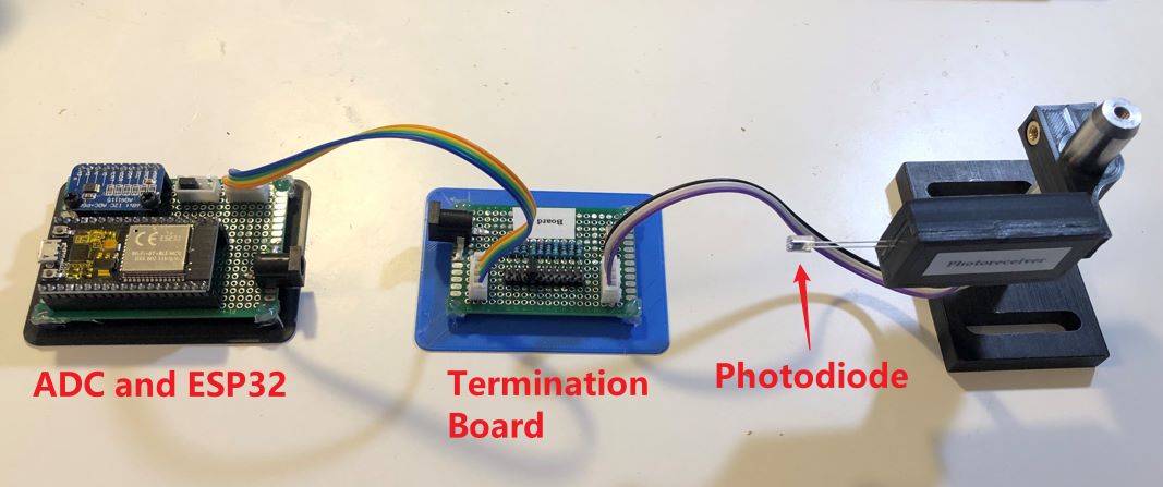
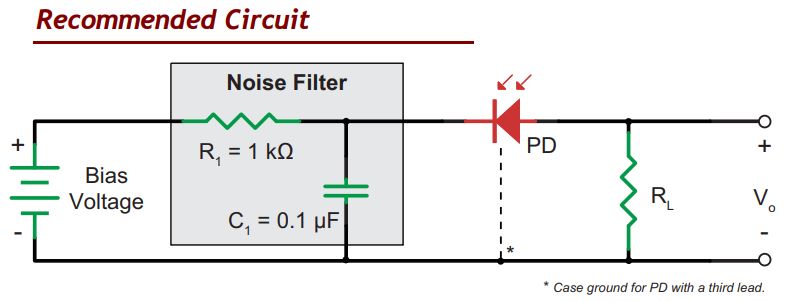
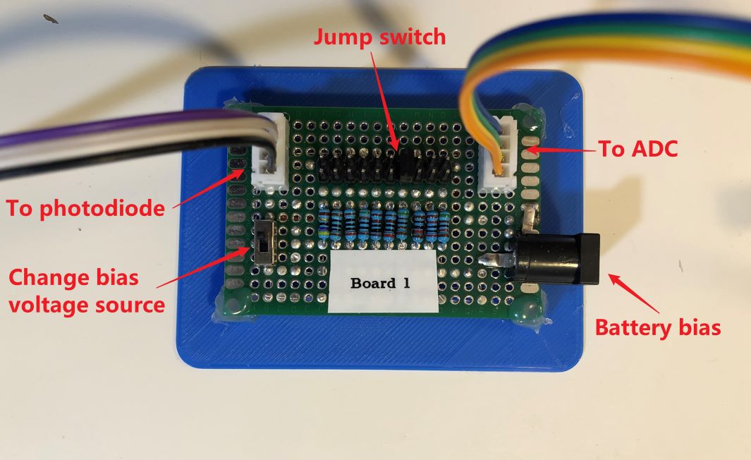
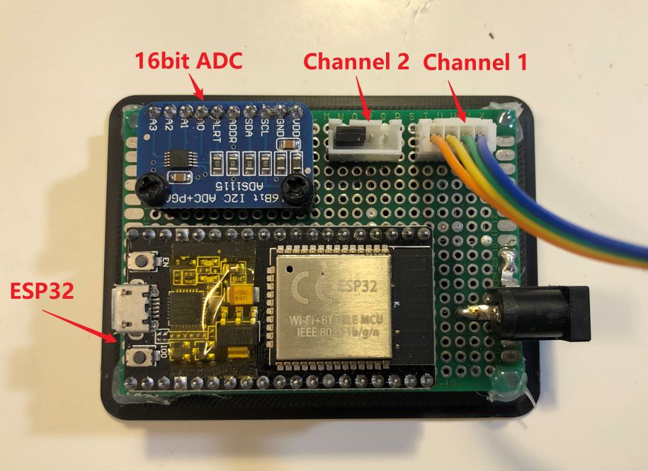
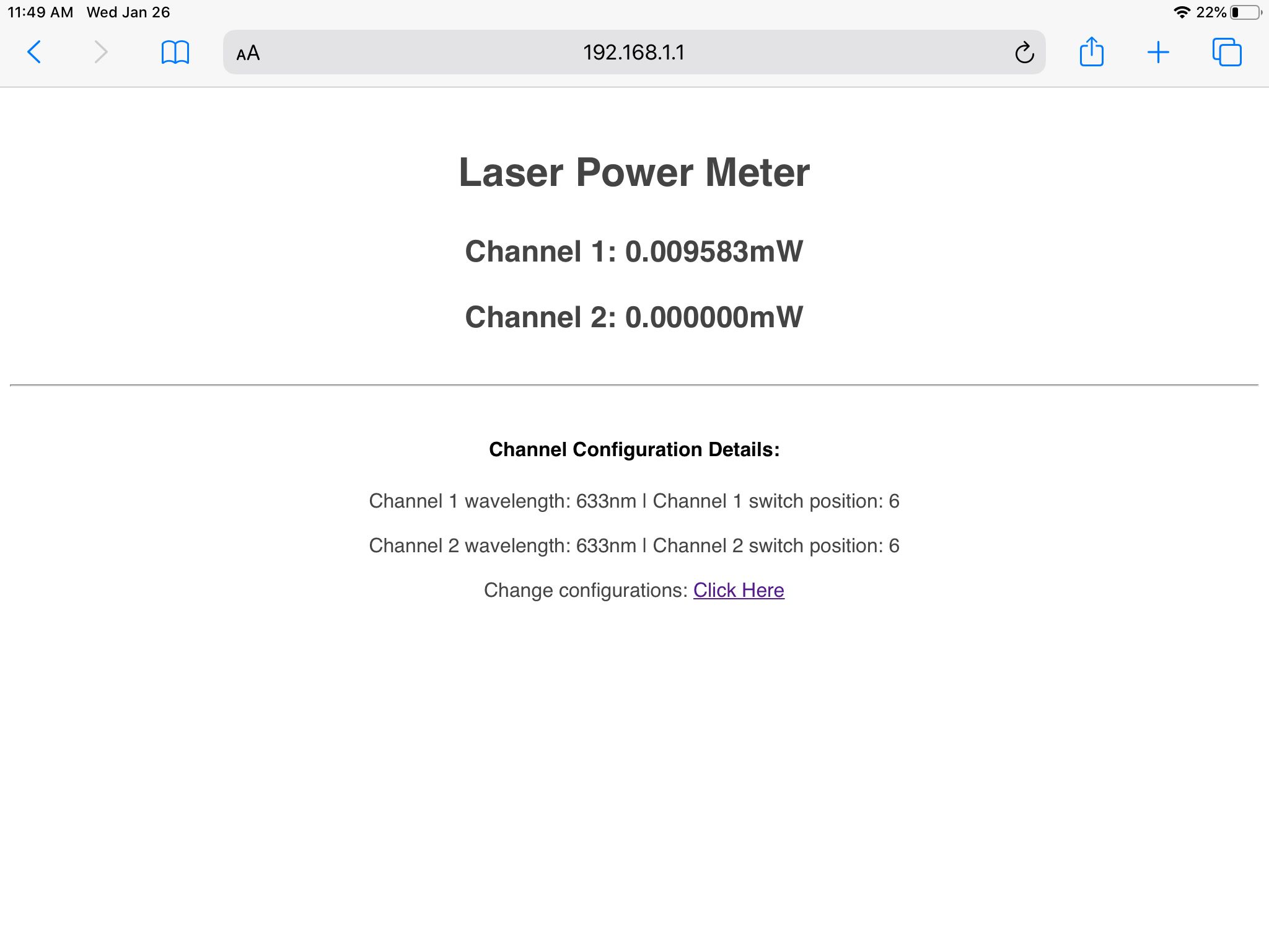
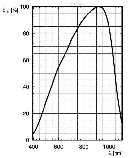
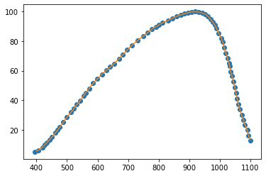
 I made a simple laser power meter. The results are pretty good. I measured my own Uniphase helium-neon laser, the results show the laser power is around 0.68 to 0.70 mW. The value is consistent with the measured results from Coherent LaserCheck. The laser power meter consists of three parts: the photodiode, termination board, and circuit board. Here is the photo of this laser power meter.
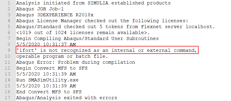
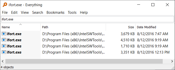
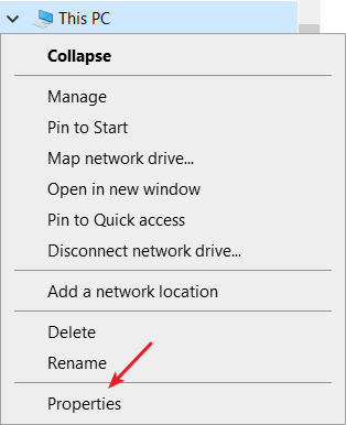
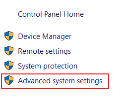
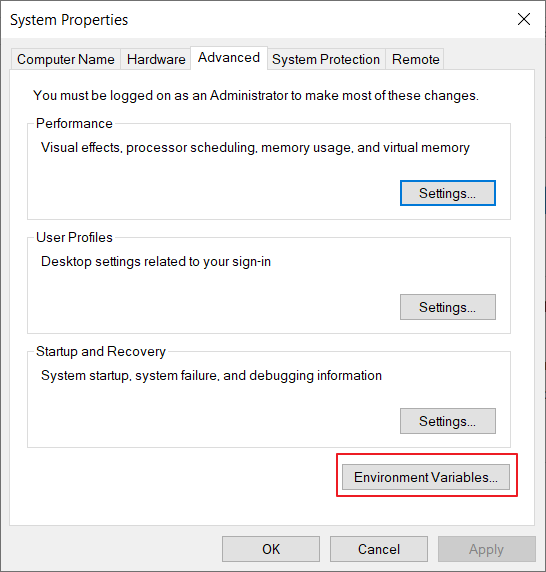
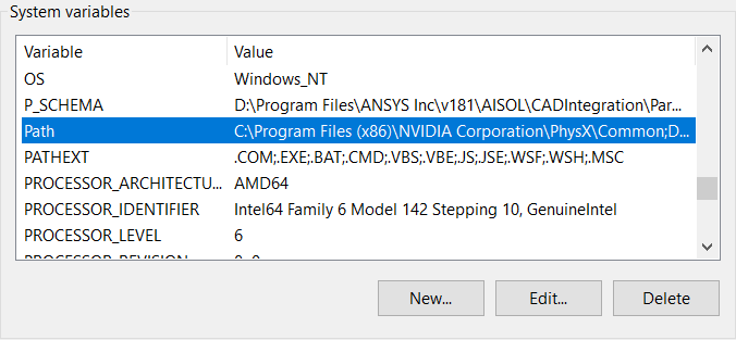
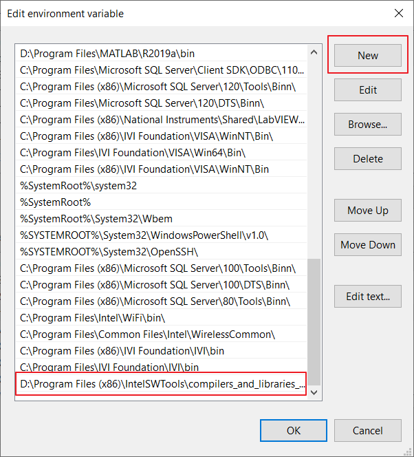
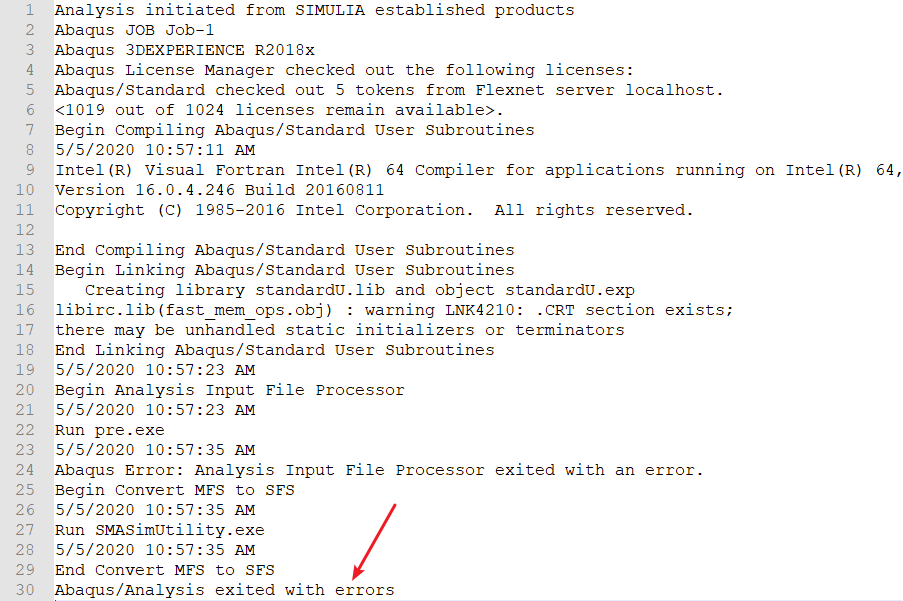
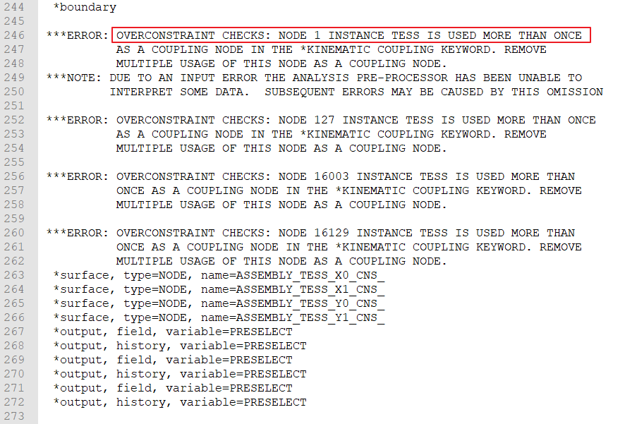
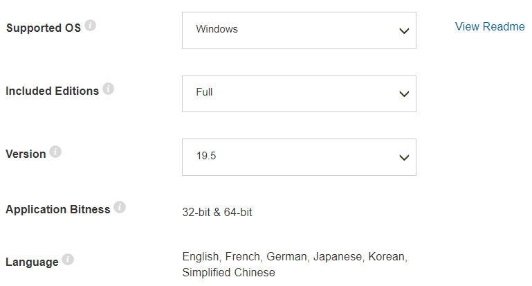
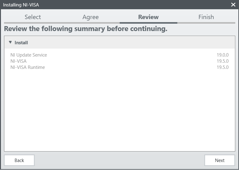
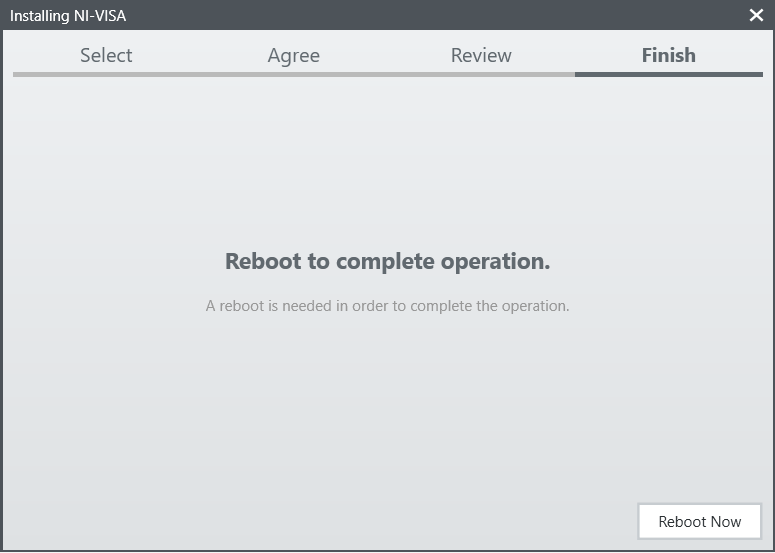
 During the subroutine environment setup, a lot of problems need to be solved. A typical problem is shown as following,
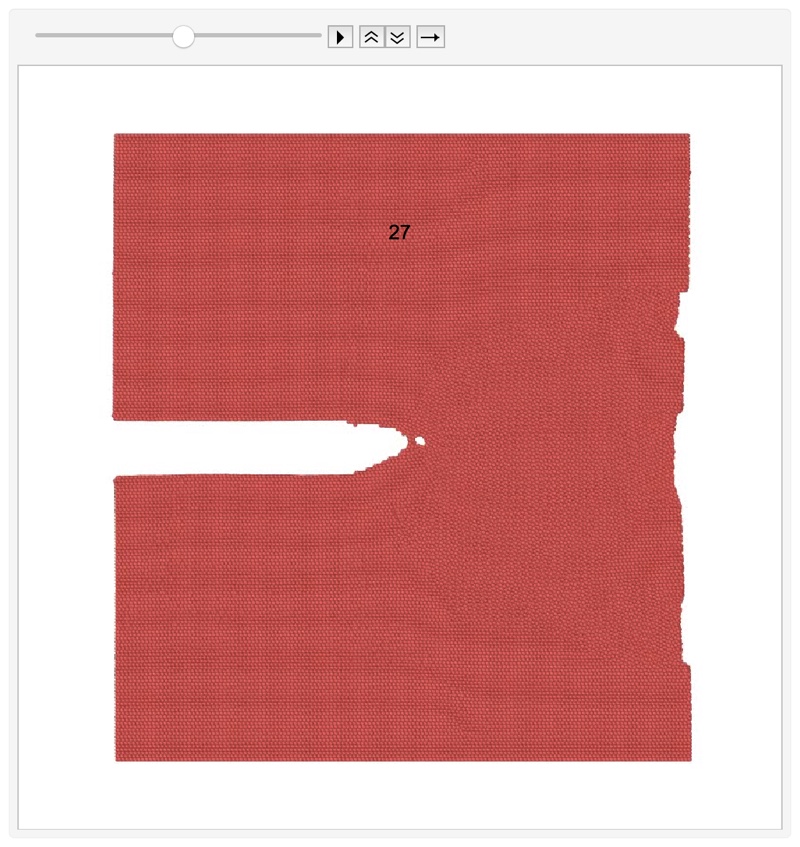
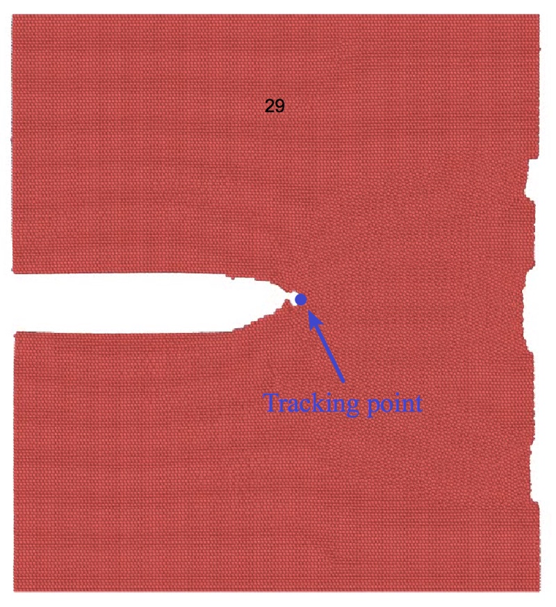
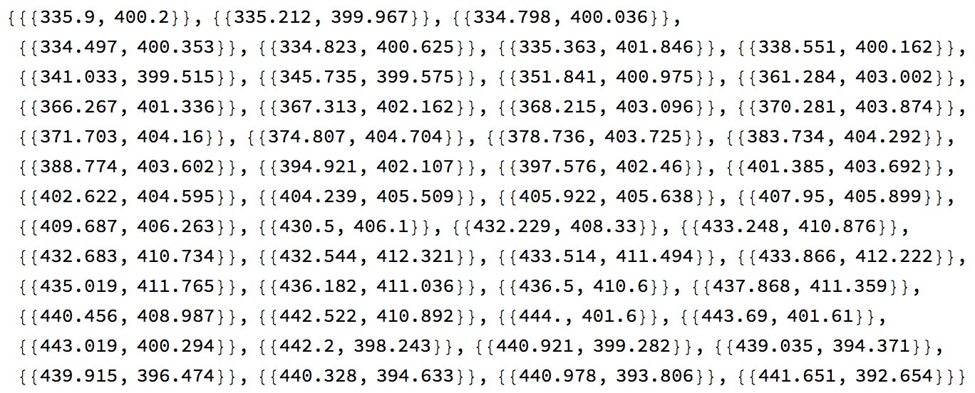
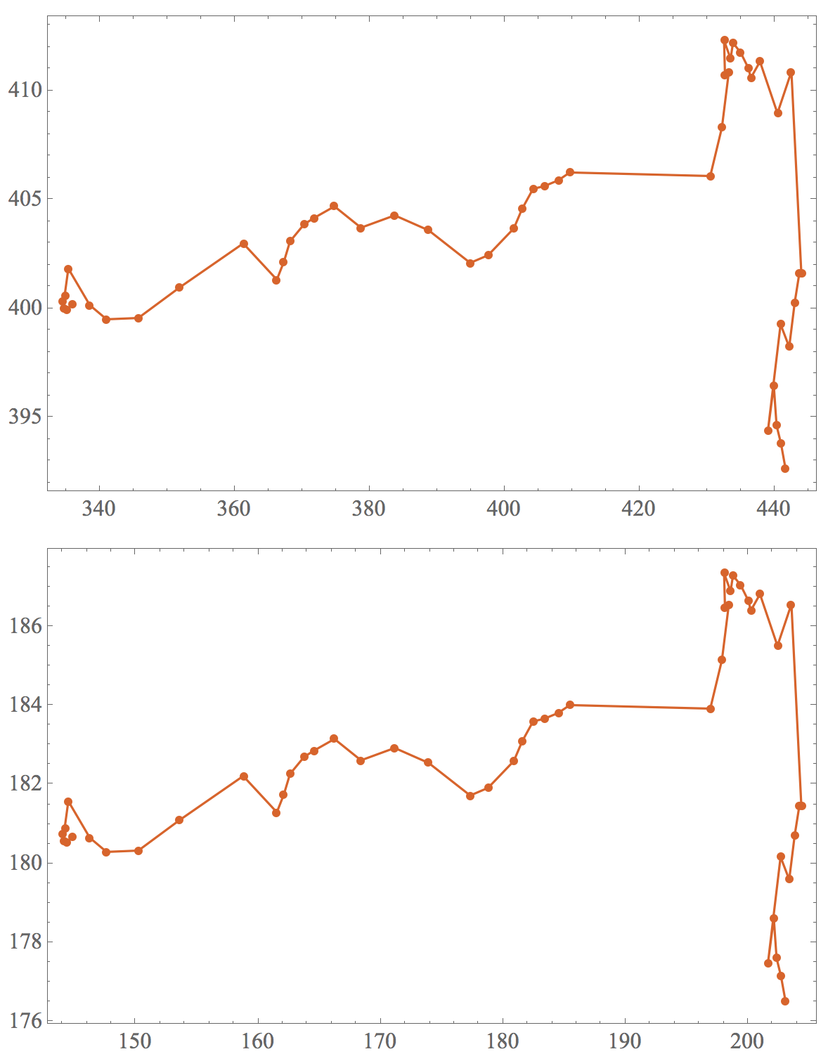
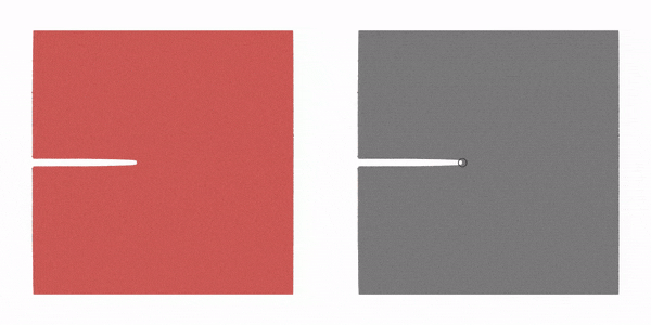
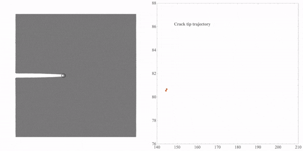
 This post focuses on the crack tip tracking method. While I simulate several fatigue models, the crack tip trajectories are hard to track in the model. Previously, I just picked some points and decided on the crack length and rate in several images. This useful method is not very effective when I get several video clips in a crack place. Several image process tools such as Fiji can deal with the image fast and easily, but I still feel it is hard to realize my goal. So I try to write a simple tool to achieve the object. Since tracking the crack tip uses the technique of image processing, I use Mathematica for this purpose.
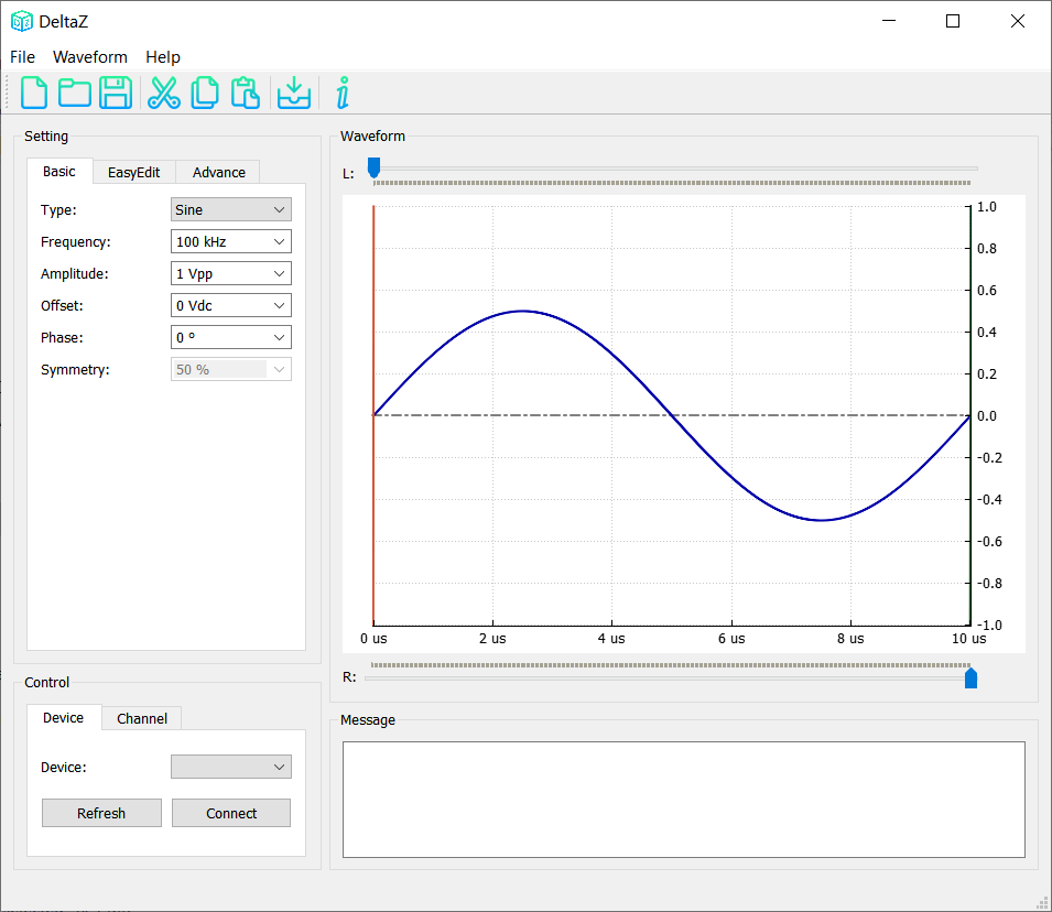
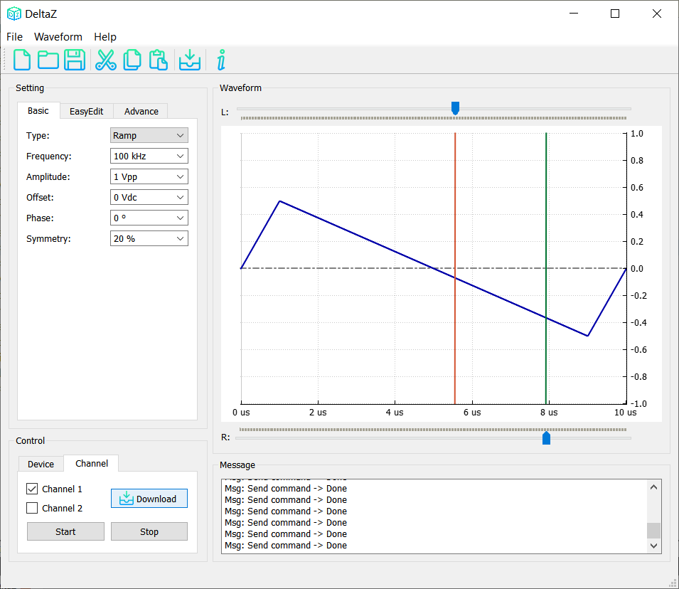
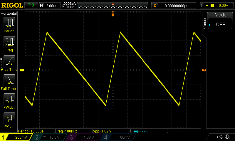
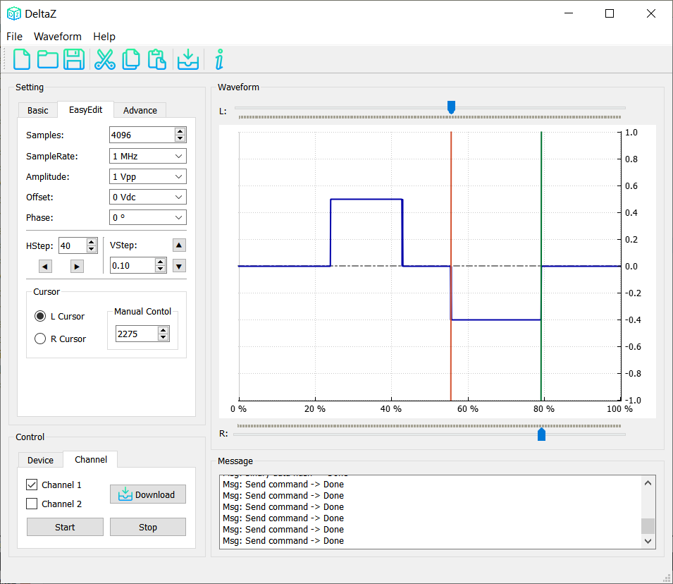
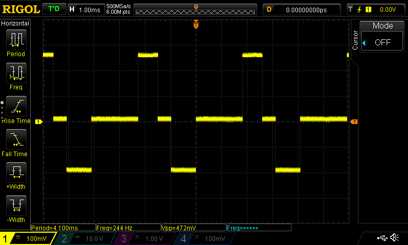
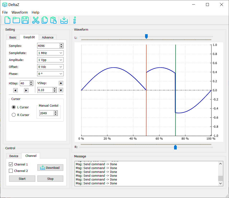
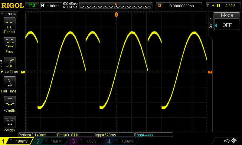
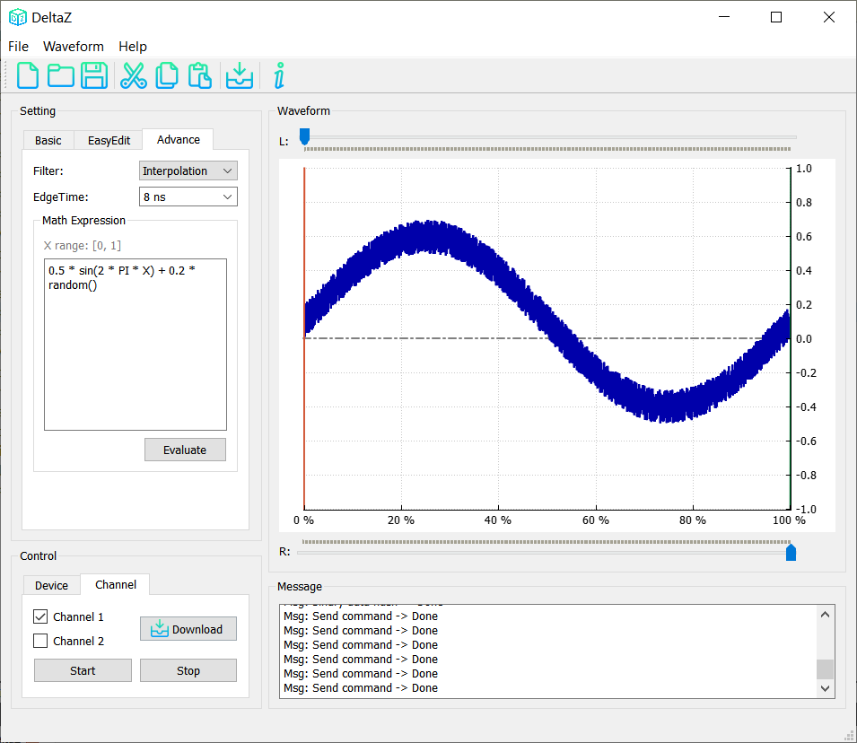
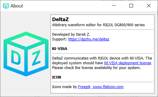
 DeltaZ is a software to edit the arbitrary waveform on RIGOL DG800/900 series. I write some scripts to control my RIGOL DG812. Finally, I decided to pack the scripts and wrote a user interface to control the device. That is DeltaZ. Click the “DOWNLOAD” button to download the software.


 LAMMPS has the capability to restart the job from the binary file. According to the description from the official website, the command restart can write out a binary restart file with the current state of the simulation every certain timestep. This command has two modes: write the binary file or the data file. If you wish to use the data file, then a convert command is needed in this scenario. Here we do not consider the data file.