 Previously, the vector space $\mathbb{V}$ and three vector product operations were considered in Simple tensor algebra I and Simple tensor algebra II. But we do not talk much about the tensor. Here, the tensor will be introduced.
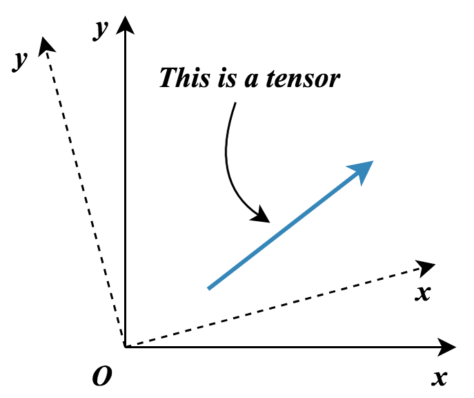
So, what is a tensor? The following figure shows a tensor in a 2D Cartesian coordinate system.
The vector is a tensor, and it is a first-order (1st-order) tensor. Actually, the scalar is a tensor as well, we can consider the scalar as a zeroth-order (0th-order) tensor.
Let $ a, b$ be two scalars in $ \mathbb{R}$, we put these two scalars (0th-order tensor) together with $ { a, b }$ to form a vector (1st-order tensor). So, if we can put two vectors $ \boldsymbol g, \boldsymbol f $ together, then we will get a 2nd-order tensor. The tensor product $ \otimes $ plays such role here ($ \boldsymbol g \otimes \boldsymbol f $).
This is not a tutorial, please refer to the books for tensor algebra.
Second-order tensor:
Let $ \mathcal{G} = {\boldsymbol g_1, \boldsymbol g_2, \boldsymbol g_3, \dots }$ and $ \mathcal{F} = {\boldsymbol f_1, \boldsymbol f_2, \boldsymbol f_3, \dots }$ be two bases in Euclidean space $ \mathbb{E}^n$. Then, the tensor product of two vectors $ \boldsymbol g_i \otimes \boldsymbol f_j $ forms a second-order tensor in $\mathbf{Lin}^n$ and it represents a basis of $\mathbf{Lin}^n$, Thus we can represent a 2nd-order tensor $ \mathbf A \in \mathbf{Lin}^n$ by,
\[\displaystyle \mathbf{A} = A^{ij} \boldsymbol g_i \otimes \boldsymbol f_j\]Then,
\[\displaystyle \boldsymbol g^i \mathbf{A} \boldsymbol f^j= \boldsymbol g^i A^{ij} (\boldsymbol g_i \otimes \boldsymbol f_j) \boldsymbol f^j = \boldsymbol g^i A^{ij} \boldsymbol g_i (\boldsymbol f_j \cdot \boldsymbol f^j) = \boldsymbol g^i A^{ij} \boldsymbol g_i (\boldsymbol f_j \cdot \boldsymbol f^j) = A^{ij}\]Similar to the dual basis in 2D vector space, four bases $ \boldsymbol g_i \otimes \boldsymbol f_j $, $ \boldsymbol g^i \otimes \boldsymbol f_j $, $ \boldsymbol g_i \otimes \boldsymbol f^j $ or $ \boldsymbol g^i \otimes \boldsymbol f^j $ are usually used in $ \mathbf{Lin}^n$. Then,
\[\displaystyle \mathbf{A} = A^{ij} \boldsymbol g_i \otimes \boldsymbol f_j = A^j_{i \cdot} \boldsymbol g^i \otimes \boldsymbol f_j= A^i_{\cdot j} \boldsymbol g_i \otimes \boldsymbol f^j = A^{ij} \boldsymbol g^i \otimes \boldsymbol f^j\]and the components
\[\displaystyle A^{ij} = \boldsymbol g^i \mathbf{A} \boldsymbol f^j\] \[\displaystyle A^j_{i \cdot} = \boldsymbol g_i \mathbf{A} \boldsymbol f^j\] \[\displaystyle A^i_{\cdot j} = \boldsymbol g_i \mathbf{A} \boldsymbol f^j\] \[\displaystyle A_{ij} = \boldsymbol g_i \mathbf{A} \boldsymbol f_j\]The identity tensor can be expressed by
\[\mathbf{I} = \boldsymbol g_i \otimes \boldsymbol g^i = \boldsymbol g^i \otimes \boldsymbol g_i = g^{ij} \boldsymbol g_i \otimes \boldsymbol g_j = g_{ij} \boldsymbol g^i \otimes \boldsymbol g^j\]where $ \boldsymbol g^i $ is dual basis of $ \boldsymbol g_i $, and,
\[\displaystyle I^{ij} = g^{ij}\] \[\displaystyle I_{ij} = g_{ij}\] \[\displaystyle I^i_{\cdot j} = I^j_{i \cdot} = \delta^i_j\]Proof: let $ \boldsymbol x \in \mathbb{E}^n$ be an arbitrary vector, \(\displaystyle \mathbf{I} \boldsymbol{x} = (\boldsymbol g_i \otimes \boldsymbol g^i)\boldsymbol{x} = \boldsymbol{g}_i (\boldsymbol{g}^i \cdot x^k \boldsymbol{g}_k) = x^i \boldsymbol{g}_i = \boldsymbol{x}\)
Tensor operations:
Previously, several operations for vectors have been introduced. The operations for 2nd-order tensor are similar to that of 1st-order tensor but there still exists some special operations defined for 2nd-order tensor or high-order tensor.
Contraction :
The contraction operation is the basic operation for a tensor. The similar concept for vectors can be found in Simple tensor algebra II. Let $ \mathbf A$ be a high-order tensor, say fourth-order tensor,
\[\displaystyle \mathbf A = A^{ij}_{\cdot\cdot kl} \boldsymbol g_i \otimes \boldsymbol g_j \otimes \boldsymbol g^k \otimes \boldsymbol g^l\]Then, the contraction means the dot product of two arbitrary bases in this tensor, say $ \boldsymbol g_j$ and $\boldsymbol g^l$,
\[\displaystyle \overset{\mathbf{Ctrc}}{\widehat{\mathbf A}} = \overset{\mathbf{Ctrc}}{ \widehat{A^{ij}_{\cdot\cdot kl} \boldsymbol g_i \otimes \boldsymbol g_j \otimes \boldsymbol g^k \otimes \boldsymbol g^l} }=\delta_j^l A^{ij}_{\cdot\cdot kl} \boldsymbol g_i \otimes \boldsymbol g^k= A^{ij}_{\cdot\cdot kj} \boldsymbol g_i \otimes \boldsymbol g^k = C^{i}_{\cdot k} \boldsymbol g_i \otimes \boldsymbol g^k\]The contraction is a basic operation for tensors. Each contraction operation will reduce the order of the tensor.
Composition:
The composition of two tensors is similar to the dot product of two vectors. Let $\mathbf A$ be the fourth-order tensor and $\mathbf B$ be the three-order tensor in $\mathbf{Lin}^n$,
\[\mathbf A = A^{ij}_{\cdot\cdot kl} \boldsymbol g_i \otimes \boldsymbol g_j \otimes \boldsymbol g^k \otimes \boldsymbol g^l\] \[\mathbf B = B^{rs}_{\cdot\cdot t} \boldsymbol g_r \otimes \boldsymbol g_s \otimes \boldsymbol g^t\]Then we use tensor product to get a result,
\[\mathbf A \otimes \mathbf B = A^{ij}_{\cdot\cdot kl} B^{rs}_{\cdot\cdot t} \boldsymbol g_i \otimes \boldsymbol g_j \otimes \boldsymbol g^k \otimes \boldsymbol g^l \otimes \boldsymbol g_r \otimes \boldsymbol g_s \otimes \boldsymbol g^t\]And contract two bases (e.g.,$ \boldsymbol g_k$ and $\boldsymbol g^s$), we get the composition result,
\[\begin{align} {\boldsymbol{AB}} &= \delta _s^k A_{ \cdot \cdot kl}^{ij}B_{ \cdot \cdot t}^{rs}{\boldsymbol{g}_i} \otimes {\boldsymbol{g}_j} \otimes {\boldsymbol{g}^l} \otimes {\boldsymbol{g}_r} \otimes {\boldsymbol{g}^t}\\ &= A_{ \cdot \cdot kl}^{ij}B_{ \cdot \cdot t}^{rk}{\boldsymbol{g}_i} \otimes {\boldsymbol{g}_j} \otimes {\boldsymbol{g}^l} \otimes {\boldsymbol{g}_r} \otimes {\boldsymbol{g}^t}\\ &= C_{ \cdot \cdot l \cdot t}^{ij \cdot r}{\boldsymbol{g}_i} \otimes {\boldsymbol{g}_j} \otimes {\boldsymbol{g}^l} \otimes {\boldsymbol{g}_r} \otimes {\boldsymbol{g}^t}\\ &= \boldsymbol C \end{align}\]The composition of two tensors satisfied the following properties:
- Associativity: $(\bf A \bf B) \bf C = \bf A (\bf B \bf C)$,
- Distributivity: $(\bf A+\bf B) \bf C = \bf A \bf C +\bf B \bf C$; $\bf A(\bf B+ \bf C) = \bf A \bf B +\bf A \bf C$.
Transposition:
The transpose operation is to change the position of the tensor index. Let $\mathbf A$ be the fourth-order tensor in $\mathbf{Lin}^n$,
\[\mathbf A = A^{ij}_{\cdot\cdot kl} \boldsymbol g_i \otimes \boldsymbol g_j \otimes \boldsymbol g^k \otimes \boldsymbol g^l\]Then,
\[\mathbf B = A^{ji}_{\cdot\cdot kl} \boldsymbol g_i \otimes \boldsymbol g_j \otimes \boldsymbol g^k \otimes \boldsymbol g^l = B^{ij}_{\cdot\cdot kl} \boldsymbol g_i \otimes \boldsymbol g_j \otimes \boldsymbol g^k \otimes \boldsymbol g^l\] \[\mathbf C = A^{\cdot ji}_{k \cdot\cdot l} \boldsymbol g_i \otimes \boldsymbol g_j \otimes \boldsymbol g^k \otimes \boldsymbol g^l = C^{ij}_{\cdot\cdot kl} \boldsymbol g_i \otimes \boldsymbol g_j \otimes \boldsymbol g^k \otimes \boldsymbol g^l\]Both are the transposed tensors of $\mathbf A$. Note that the transposition do not change the permutation of the bases.
Decomposition:
Follow the rule in Transposition, and consider the fourth-order tensor $\mathbf A$ and its transposed tensor $\mathbf A^ \text T$,
\[{\bf{A}^\text T} = A_{ \cdot \cdot kl}^{ji}{\boldsymbol {g}_i} \otimes {\boldsymbol {g}_j} \otimes {\boldsymbol {g}^k} \otimes {\boldsymbol {g}^l}\]If,
\[A_{ \cdot \cdot kl}^{ji} = A_{ \cdot \cdot kl}^{ij}\]Then, the fouth-order tensor is a symmetric tensor with respect to the first and second index. If the tensor $\mathbf A$ and its transposed tensor $\mathbf A^ \text T$ satisfy,
\[A_{ \cdot \cdot kl}^{ji} = -A_{ \cdot \cdot kl}^{ij}\]Then, the tensor $\mathbf A$ is skew-symmetric with respect to the first and second index. All the elements on the diagonal of a skew-symmetric matrix are zero, we use the following notation,
\[A_{ \cdot \cdot kl}^{\underline i \underline i } = 0\]The underlinded symbol means no summation convention for index $i$.
Now, the symmetric and the skew-symmetric tensor can be constructed by the tensor and its transposed tensor,
\[{\bf{D}} = \frac{1}{2}\left( {\bf{A} + {\bf{A}^{\rm{T}}}} \right)\] \[{\bf{W}} = \frac{1}{2}\left( {\bf{A} - {\bf{A}^{\rm{T}}}} \right)\]Stress:
Here, we consider the stress tensor in three dimensional space as an example,
\[{\boldsymbol{ \sigma }} = {\sigma _{ij}}{\boldsymbol e_i} \otimes {\boldsymbol e_j} = \left[ {\begin{array}{cc} {\sigma _{11}}&{\sigma _{12}}&{\sigma _{13}}\\ {\sigma _{21}}&{\sigma _{22}}&{\sigma _{23}}\\ {\sigma _{31}}&{\sigma _{32}}&{\sigma _{33}} \end{array}} \right]\]With the given direction $\boldsymbol n=n^i \boldsymbol e_i$ (unit vector), the traction vector is given by,
\[{\bf T = \boldsymbol \sigma \cdot \boldsymbol n}\]and the normal stress on this surface can be written by,
\[{\sigma _n} = \bf T \cdot \boldsymbol n =\boldsymbol n \cdot \boldsymbol \sigma \cdot \boldsymbol n\]Then, we decompose the stress into two tensors,
\[{\boldsymbol{\sigma }} = sph({\boldsymbol{\sigma }}) + dev({\boldsymbol{\sigma }})\] \[sph({\boldsymbol{\sigma }}) = \frac{1}{3}{\rm{Tr}}({\boldsymbol{\sigma }}){\bf{I}};dev({\boldsymbol{\sigma }}) = {\boldsymbol{\sigma }} - \frac{1}{3}{\rm{Tr}}({\boldsymbol{\sigma }}){\bf{I}}\]$sph({\boldsymbol{\sigma }})$ is the hydrostatic part of the stress and $dev({\boldsymbol{\sigma }})$ is the deviatoric part of the stress. Hydrostatic stress is about the volumn change and the Deviatoric stress is corresponded to the plastic deformation.