 This is a homework of computational nanomechanics. The basic requirement is to use the Lagrangian function to describe the motion of particles. In homework, it requires 5 particles. As an enhancement, I rewrote the code with Qt and use GNU Scientific Library(GSL) to finish the task.
Concept
The Lagrangian equation of motion describe the particle motion with energy method, the equation is:
\[\displaystyle \frac{d}{dt}\frac{\partial L}{\partial \dot{x}_k}-\frac{\partial L}{\partial x_k}=0\]$ L$ is the Lagrangian function of the system, $ k$ denotes the degree of freedom.
\[\displaystyle L = T - U\]$ T$ is the kinetic energy and $ U$ is the potential energy.
Since the derivative of $ U$ with respect to $ x$ is the force
\[\displaystyle f = -\frac{dU(r)}{dr}\]the Lagrangian equation of motion uses another way to illustrate Newton’s second law.
Single particle example
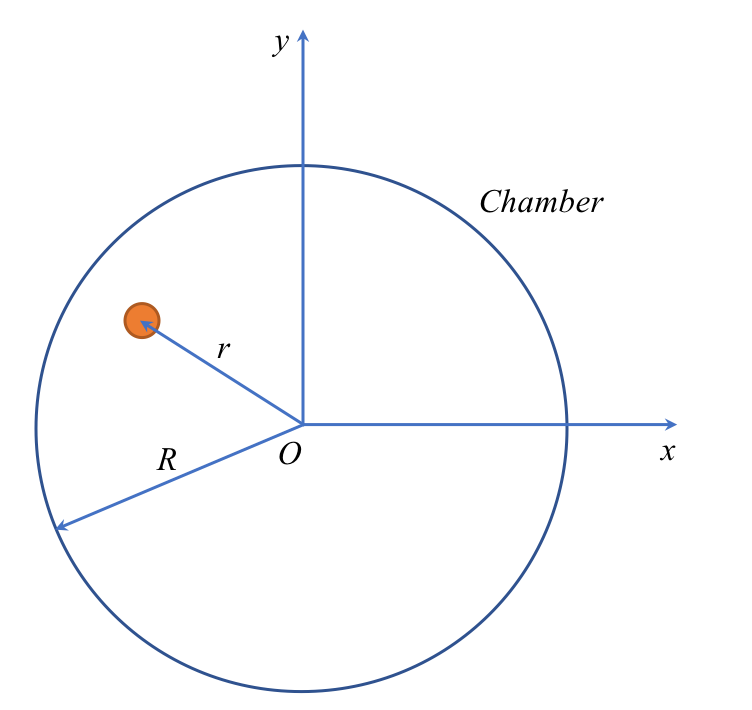
For a single particle in a chamber, two degree of freedom $ x_1 = x, x_2 = y$, the kinetic energy is:
\[\displaystyle T =\sum \frac{1}{2} m \left({\dot{x}}^2 + {\dot{y}}^2\right)\]$ k$ is the degree of freedom. $ m$ denotes the mass of the particle.
The potential energy of the particle in a chamber is expressed as:
\[\displaystyle U = \alpha e^{- \beta(R-r)}\]Here the exponent function is used to describe the repulsion from the chamber wall. when the distance $R-r$ close to zero, the repulsion potential will be much large and prevent the particle penetrating the chamber wall. The Lagrangian function and equations are:
\[\displaystyle L = \frac{m}{2} (\dot{x}^2+\dot{y}^2)-\alpha e^{-\beta (R-\sqrt{x^2+y^2})}\]and for each degree of freedom:
\[\displaystyle \left\{\begin{matrix} m \ddot{x}(t) = -\alpha \beta e^{-\beta (R-\sqrt{x^2+y^2})} x(t) / \sqrt{x^2+y^2} \\ m \ddot{y}(t) = -\alpha \beta e^{-\beta (R-\sqrt{x^2+y^2})} y(t) / \sqrt{x^2+y^2} \end{matrix}\right.\]For this example, we take the following parameters:
\[\displaystyle \alpha = 10^{-27}, \beta = 4nm^{-1}, R = 10nm, m = 10^{-9}kg\]The initial conditions are:
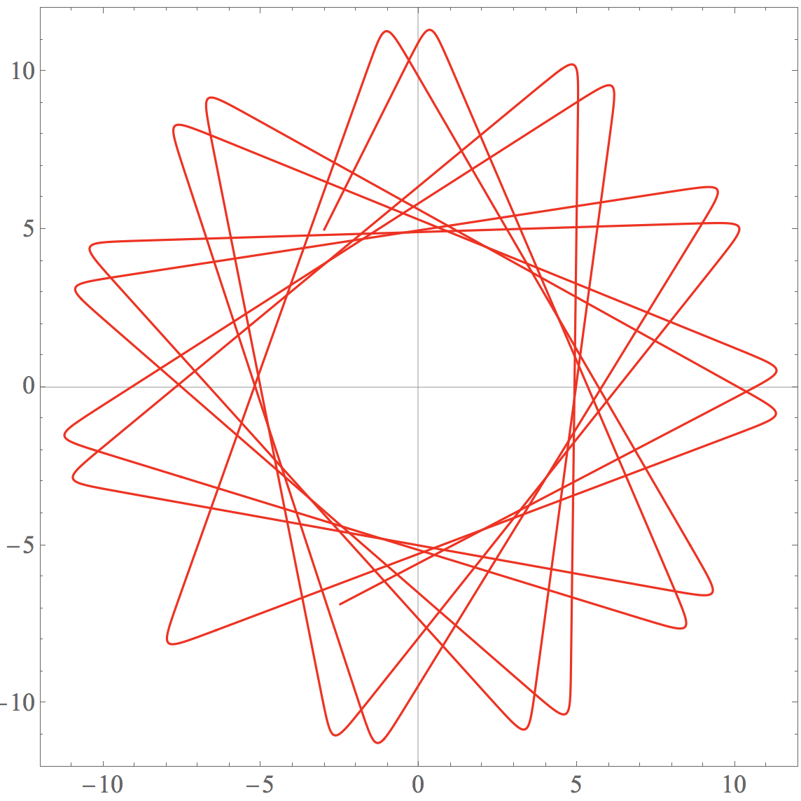
\[\displaystyle x(0) = -3nm, \dot{x}(0) = 10nm/s, y(0) = 5nm, \dot{y}(0) = 20nm/s\]Using Mathematica (MDSimulation1.nb) to plot the trajectory or use this script (MDSimulation2.nb) to plot the animation,
Lennard-Jones potential function
Lennard-Jones potential function is almost the world-famous potential function in nano mechanics. It describes the interaction between atoms. The function was proposed through quantum perturbation theory in which the attraction should follow a $r^{6}$ relation. It combines the attraction and repulsion together.
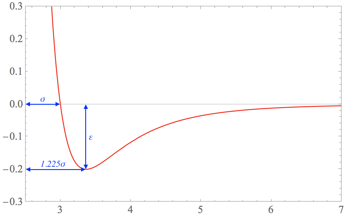
\[\displaystyle U(r_{ij})=4 \varepsilon \left[ \left(\frac{\sigma}{r_{ij}} \right)^{12} - \left( \frac{\sigma}{r_{ij}}\right)^{6} \right]\]where: $ \varepsilon$ denotes the depth of the energy well, and $ \sigma$ denotes the equilibrium spacing of atoms.
Take $ \sigma = 3, \varepsilon = 0.2$, the result is shown below,
As mentioned before, the derivative of $ U$ with respect to $r$ is the force. The force from Lennard-Jones interaction is simply get the derivative of $ U$:
\[\displaystyle F=-U^{\prime}(r_{ij}) = -4 \varepsilon \left(\frac{6 \sigma ^6}{r^7}-\frac{12 \sigma ^{12}}{r^{13}}\right)\]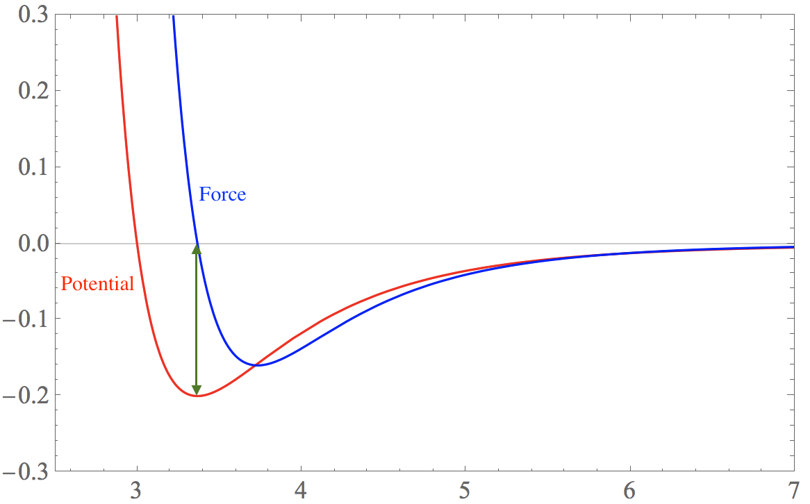
The equilibrium distance between two atoms is the position $ F=0$.
\[\displaystyle \sigma \sqrt[6]{2} = r_0\] \[\displaystyle r_0 = 1.225 \sigma\]Two particles example
If two particles are put into the chamber, Lennard-Jones potential should be considered in the calculation. Here, I try to use GNU Scientific Library(GSL) to solve the problem in three dimensions.
The Explicit 4th order (classical) Runge-Kutta(RK4) method is chosen for this problem. Two particles are denoted as $i$ and $ j$ respectively. The Lagrangian function is ($ k$ denotes the degree of freedom):
\[\displaystyle L=T-U\] \[\displaystyle T = \sum \frac{1}{2}m_i (\dot{x}_{ik}^2)+\sum \frac{1}{2}m_j (\dot{x}_{jk}^2)\] \[\displaystyle U = E_{pi} + E_{pj} + W_{LJ}\]$ E_{pi}$ and $ E_{pj}$ denotes the repulsive potential from the chamber wall, the equations of them are similar to Single particle example. Here, I just analyze the Lanner-Jones potential:
\[\displaystyle W_{LJ-ijk} = 4 \varepsilon \left[ \frac{\sigma ^ {12}}{\left(\sum_{k=1}^3 \left( x_{ik} - x_{jk}\right)^2 \right)^6} - \frac{\sigma ^ 6}{\left(\sum_{k=1}^3 \left( x_{ik} - x_{jk}\right)^2 \right)^3} \right]\]For the derivative $ W_{LJ-ijk}$ with respect to $ x_{ik}$ and $ x_{jk}$:
\[\displaystyle \frac{\partial W_{LJ-ijk}}{\partial x_{ik}} = 4 \varepsilon \left[ \frac{6 (x_{ik}-x_{jk})\sigma ^ {6}}{\left(\sum_{k=1}^3 \left( x_{ik} - x_{jk}\right)^2 \right)^4} - \frac{12 (x_{ik}-x_{jk}) \sigma ^ {12}}{\left(\sum_{k=1}^3 \left( x_{ik} - x_{jk}\right)^2 \right)^7} \right]\] \[\displaystyle \frac{\partial W_{LJ-ijk}}{\partial x_{jk}} = 4 \varepsilon \left[ -\frac{6 (x_{ik}-x_{jk})\sigma ^ {6}}{\left(\sum_{k=1}^3 \left( x_{ik} - x_{jk}\right)^2 \right)^4} + \frac{12 (x_{ik}-x_{jk}) \sigma ^ {12}}{\left(\sum_{k=1}^3 \left( x_{ik} - x_{jk}\right)^2 \right)^7} \right]\]With these two equations, we can simply calculate the motion of these two particles,