 This post focuses on the crack tip tracking method. While I simulate several fatigue models, the crack tip trajectories are hard to track in the model. Previously, I just picked some points and decided on the crack length and rate in several images. This useful method is not very effective when I get several video clips in a crack place. Several image process tools such as Fiji can deal with the image fast and easily, but I still feel it is hard to realize my goal. So I try to write a simple tool to achieve the object. Since tracking the crack tip uses the technique of image processing, I use Mathematica for this purpose.
The main function used in Mathematica is the function called “ImageFeatureTrack”. This function will track some feature points in a sequence of images, and return the coordinates of these points in each image. Thus, the idea is not very difficult, we import the video and transfer it into the image sequence, then we specify the tracking points with the coordinates in the image and use ”ImageFeatureTrack” function to get the coordinates in each frame. The last step is to turn the image coordinates into the real model coordinates.
The first step is to import the file and turn it into a sequence of images. Additionally, the frame numbers are added to each frame to help inspect the image sequence,
1 | |
The last line uses the “ListAnimate” command to generate a generate animation in Mathematica,
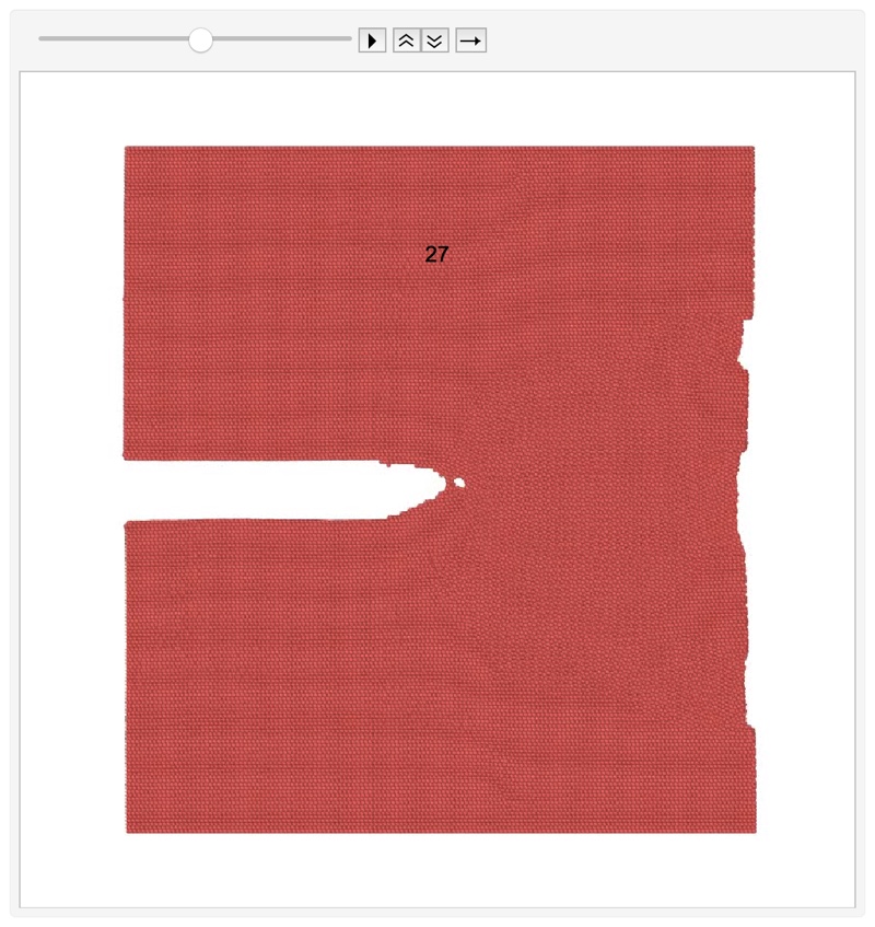
Then, the tracking frame should be set according to the animation, in this example, the crack has a jump in 28th to 29th frame, so the frame number 29 should be used. At the end of the simulation, the crack becomes much more width, so I select more frames here,
1 | |
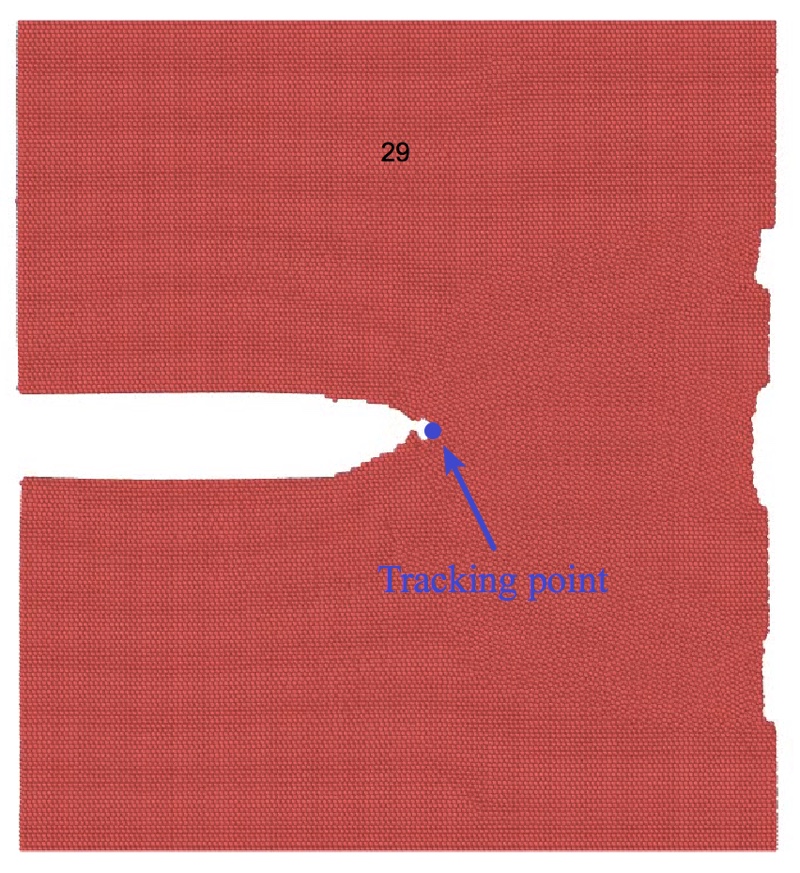
The 1st, 29th, 38th, 42nd are shown to select the feature points here. Right-click the image and select Get Coordinates tool in the menu and pick the feature points on the image. Then use “Edit”->”Copy” to copy the coordinates. Since we chose four frames for tracking, four crack-tip feature points should be chosen. The following figure shows the point that I chose in the 29th frame.
Paste the coordinates into the following code,
1 | |
The image coordinates of the crack tip will be stored in rST1,
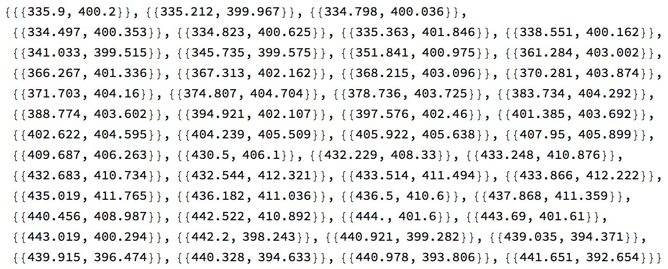
Note that all these coordinates are just the image coordinates directly calculated from the image. Before we turn these coordinates into the real coordinates in the model, we should check the tracking quality. The method is very simple, I draw a small blue circle with the coordinates in “rST1” to each frame,
1 | |
Drag the slide bar to check the tracking quality. If Mathematica lost the tracking point, you should add more tracking frames in the previous code to correct the result. If the crack tip trajectory is tracked correctly, then the following code is used to transfer the image coordinates into the real coordinates in the model,
1 | |
To calculate the real coordinates, I use the coordinates of two points. “realCoord” stores the real coordinates in the model, and “imgCoord” stores the coordinates in the image at the same model position. The result will be saved in rST2. Two list plots will be drawn to compare the coordinates,
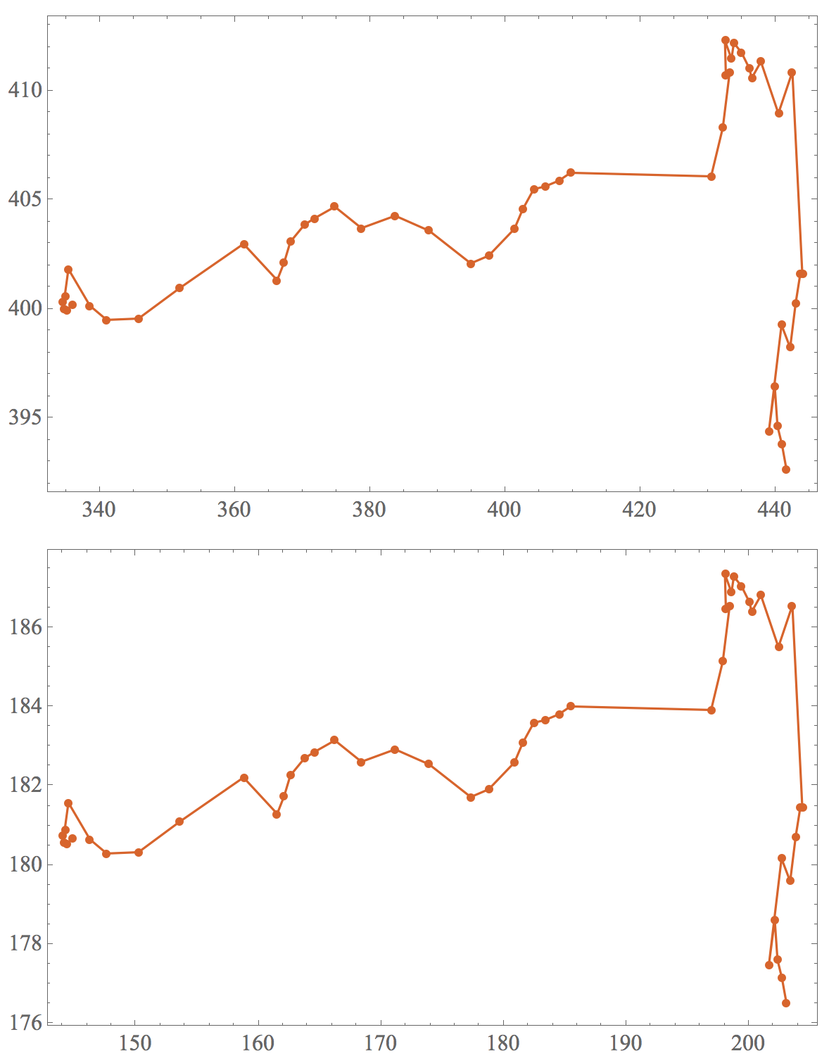
The first figure is about the image coordinates and the second figure is the real coordinates in the model. Then, we export the animation.
1 | |
Here is the result animation: