 Previously, I developed a extraction tool for hysteresis curve data but decided to rewrite it for two main reasons. Firstly, the Python packaging program could only be used on a 64-bit platform, and secondly, pre-processing for the images was somewhat cumbersome. Thus, I redeveloped this image data extraction software using C++ combined with OpenCV. The software employs OpenCV’s simplest color recognition method, along with dilation and erosion functions, allowing for effective extraction of curve data from images, including logarithmic coordinate extraction now.
Download and Installation
The software is compatible with Windows (x32, x64) platforms: DOWNLOAD
Basic Operation
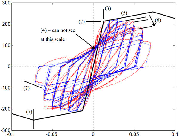
For simplicity, let’s test data extraction using the following image, aiming to extract the blue curve data points,
Note: The image is included in the software installation directory with the name
Img.png. To enhance web transmission speed, the image has been compressed.
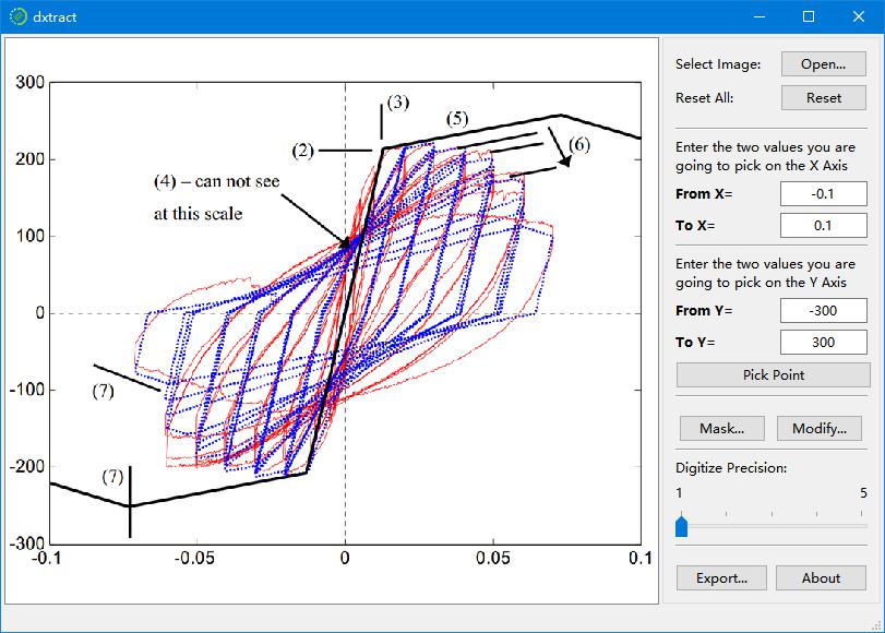
Upon opening the software and loading the curve image, the image area allows for scroll wheel zooming and left-click panning. Double left-clicking and right-clicking will be used during the point selection process,
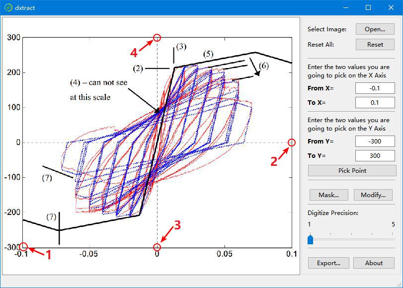
After setting the start and end coordinates in “From X”, “To X”, “From Y”, and “To Y”, click “Pick Point”. The cursor will change to a crosshair. Right-click or double-click on the four points in the image corresponding to X=-0.1, X=0.1, Y=-300, and Y=300 (though you don’t have to choose precisely these points). Pay attention to the status bar for prompts during the selection process,
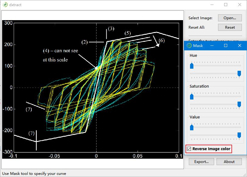
Afterwards, the “Pick Point” button and the input fields above will be disabled until you click “Reset” to restart the extraction process. Next, add a “Mask” to the image to cover unwanted parts in black, leaving only the data to be extracted. The software will extract all data from non-pure black parts of the image. If the curve is black or dark, you can invert the colors in “Mask…”. Click the “Mask…” button to open the HSV color control dialog. Since the blue data points are dark and the background is white, first check the “Reverse Image Color” option. The image colors will invert, turning the blue curve into a yellow one,
Adjust each slider in the HSV color control dialog, trying to minimize the distance between the “Hue”, “Saturation”, and “Value” sliders while ensuring the yellow curve remains. This not only removes extraneous colors but also reduces the number of noise pixels in the image (Tip: If the extraction results with many noise pixels or the noise matches the curve color, use the “Erode” function in “Modify…” to remove noise, then “Dilate” to restore the eroded curve),
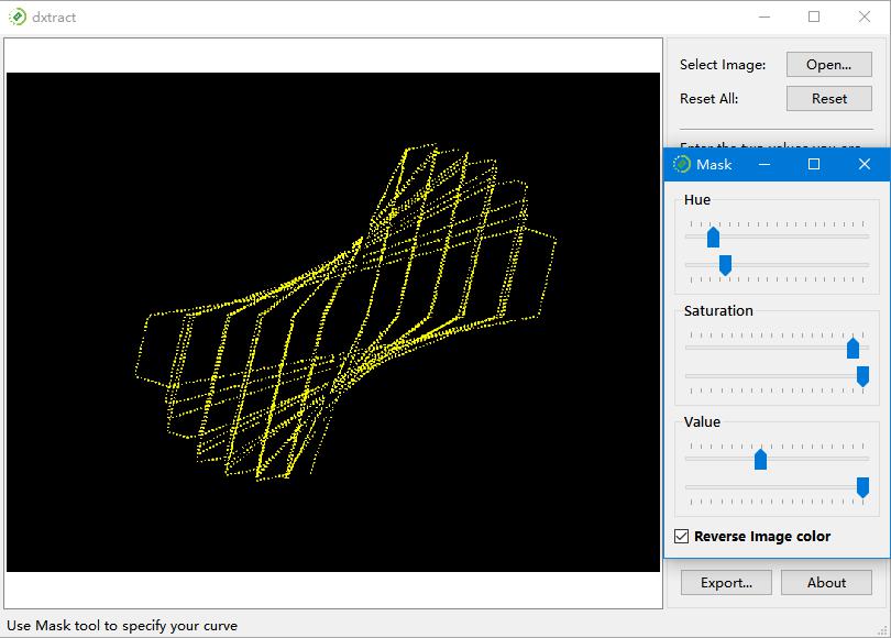
Adjust the sliders to the positions shown above (specific adjustments may require several attempts) to ensure only the desired curve remains on the image. Close the HSV color control dialog, set “Digitize Precision” to control image sampling precision — 1 for highest precision, 5 for lowest. Default is 1, but if the image is large and yields many data points, increasing the “Digitize Precision” value can reduce the amount of sampled data. Default here is 1, click “Export…”,
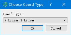
For standard axes, select “X: Linear Y: Linear”. For logarithmic coordinates, choose the respective logarithmic option for the X or Y axis from the dropdown menu. Following the default settings, click OK, then choose a location to save the CSV data. Open the CSV file in Excel, select the two columns of data, and plot a scatter graph,
The extraction result is as follows,
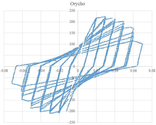
From the figure, it is evident that all parts of the curve not obscured by other lines have been extracted. While the software can’t infer obscured parts of the curve, it’s generally sufficient for most purposes.