 Previously, when I analyzed a steel structure with residual stress, it is difficult to apply residual stresses correctly and could not identify the problem until I came across a case study on applying residual stresses. In Ansys, initial stresses can be considered as a load but are only applicable in static and transient analyses. Constant initial stresses can be applied using the ISTRESS command.
In practice, however, initial stresses are generally applied using an initial stress file that stores the actual distribution of initial stresses within the structure. This file can be obtained through calculations of residual stress distribution based on initial stresses from previous loads. The ISFILE command is used to read this file, where the LOC variable within the ISFILE command specifies the initial residual stresses read from the file to be applied to elements or integration points. For element centroids, LOC defaults to 0, for integration points, LOC can be set to 1, and setting LOC to 2 allows specifying different initial stress positions for each individual element. In this case, the initial stress file should provide a stress position identifier for each element’s initial stress. When LOC=3, the initial stress state is the same for every element in the specified mesh.
This post involves a simplified model of a rock layer under the gravity and uniform pressure. The model is analyzed by general analysis and initial stress analysis.
General Analysis
The general analysis directly applies gravity and uniform pressure. The finite element model is shown in the following figure,
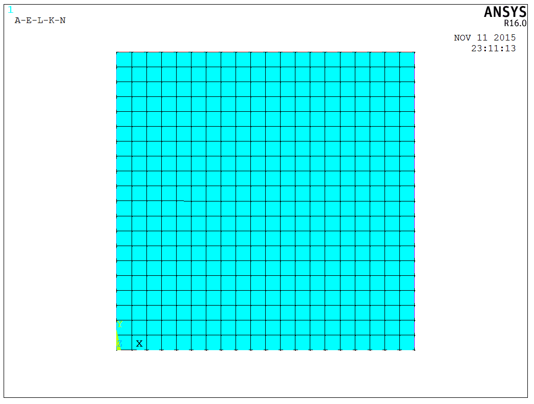
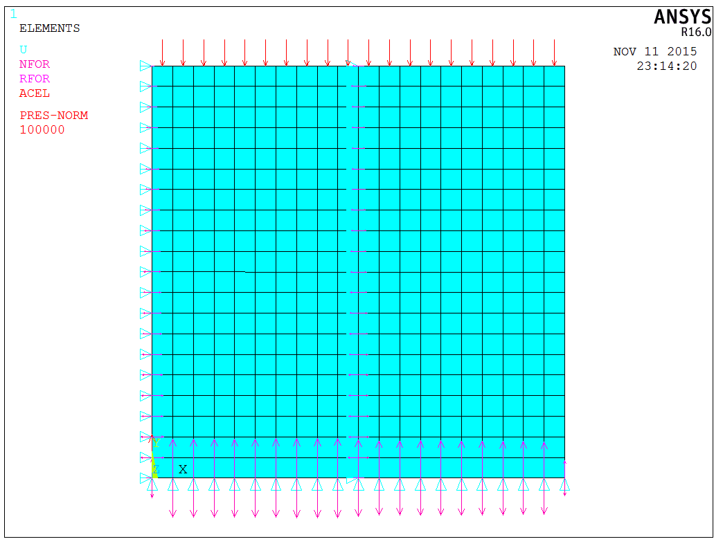
The rock layer is 2×2m. Considering the computational cost, the model is simulated by PLANE42 elements, with material as elastic. The top has a uniform lithostatic pressure of 1E5Pa, in addition to gravity load. The structure is constrained at the bottom vertically and horizontally on the sides. The load applied to the structure is as shown in the following figure,
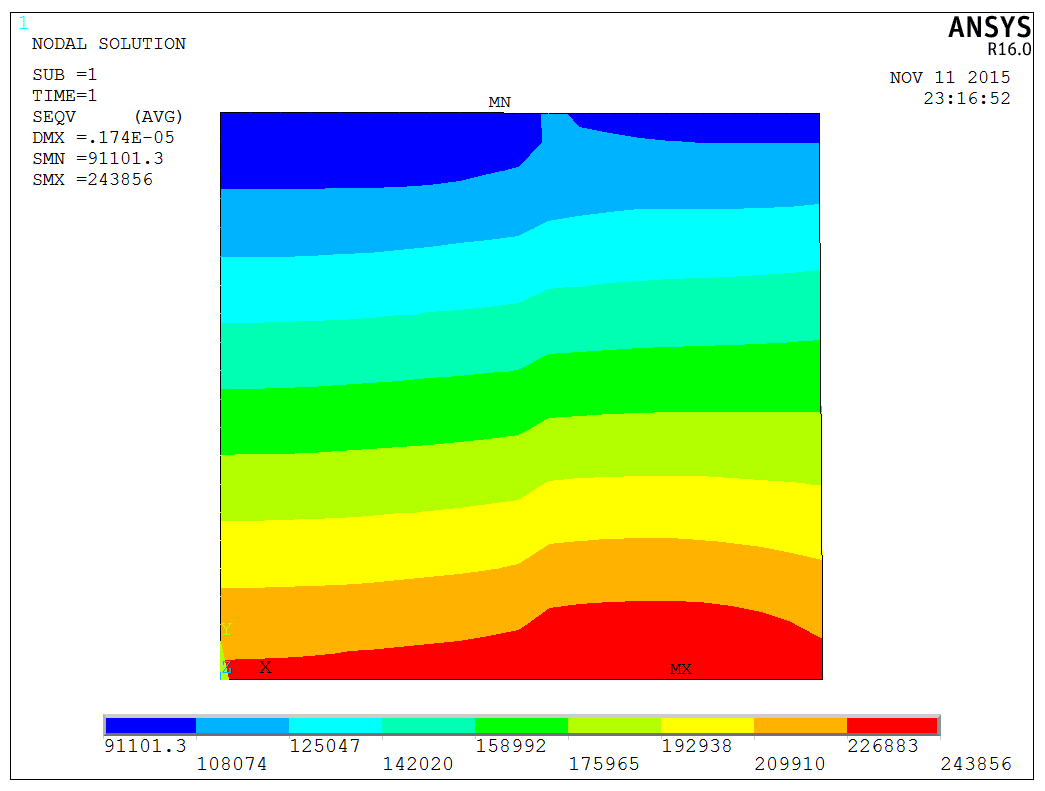
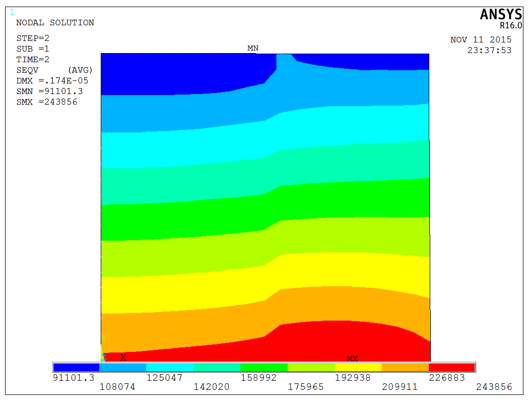
By directly solving provides the structure’s equivalent stress distribution, as shown in the following figure,
Initial Stress Analysis
The idea behind initial stress analysis is to generate initial stresses from gravity, write them into an initial stress file. Then we can recreate the model, fix all elements and nodes, read and apply the initial stress file. Afterwards, we capture all nodal reactions, write these reactions into a file, recreate the model, and solve by applying nodal reactions and corresponding uniform pressure.
This process is somewhat cumbersome for this model, mainly because the initial stress originates from an actual solution. Usually, the initial stress file might be directly provided, obtained from experiments or calculated based on formulas, thus understanding the specific steps for applying initial stresses is crucial here.
Step 1
Create the model and apply the gravitational field, which is similar to the above steps. Then use ISWRITE,1 before solving the model to write the calculated initial stresses into a Jobname.ist file, as shown in the following figure,
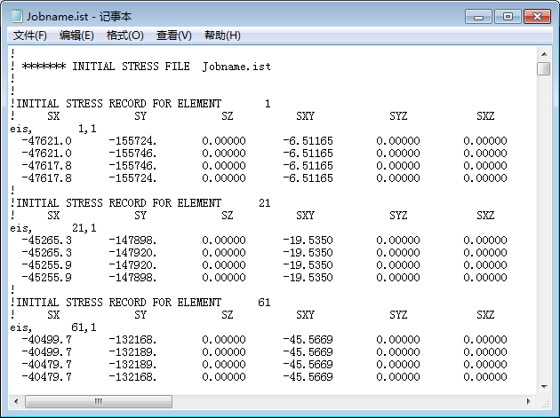
The standard initial stress file starts with comment lines “!”, followed by a record for each element starting with the string “EIS”, then the element number and optional position indicator, separated by “,”, followed by the stress records for the element.
Step 2
Rebuild the model, constrain all nodes, and apply the initial stresses with the following statementl
1 | |
The following command can list the applied initial stresses,
1 | |
Then we can solve the model directly. This leads to a Jobname2.rst file, the result file after applying the initial stress file in step 2, which will be used in step 3.
Step 3
Rebuild the model again, apply uniform pressure load, and use the following command to apply the corresponding equivalent nodal forces,
1 | |
After solving the model, the equivalent stress distribution is obtained as follows,
By comparing the final contour distributions from both analyses, we can find they show the same results, indicating the correct application of initial stresses.
The model is a test model, and the APDL code is available upon request.