 During structural analysis, it is common to use multiple types of elements together. This leads to issues related to the connection between elements. General elements like beams, shells, and solid elements usually connect via shared nodes. However, due to the differences in degrees of freedom (DOF) between elements, such connections might not yield the desired results and can even lead to issues that prevent model convergence. Thus, it is necessary to create “compatibility conditions” between different elements.
Constraint equations are a commonly used method to create “compatibility conditions,” with their basic form as follows:
\[Constant = \sum\limits_{I = 1}^N {\left( {Coeff\left( I \right) \times U\left( I \right)} \right)}\]where $U(I)$ is the DOF item, $Coeff(I)$ is the coefficient of the DOF, $N$ is the term number in the equation.
In ANSYS, the CE command is used to apply constraint equations, which has the following format,
1 | |
where:
- NEQN is the constraint equation reference number, which can be:
- N: Arbitrary set number.
- HIGH: The highest defined constraint equation number. This option is especially useful when adding nodes to an existing set.
- NEXT: The highest defined constraint equation number plus one. This option automatically numbers coupled sets so that existing sets are not modified.
- By default, it is HIGH.
- CONST is the constant term of the equation.
- NODE1 is the node number for the first term of the constraint equation. Using -NODE1 removes that term.
- Lab1 is the DOF identifier for the node, Structural labels: UX, UY, or UZ (displacements); ROTX, ROTY, or ROTZ (rotations, in radians). Thermal labels: TEMP, TBOT, TE2, TE3, . . ., TTOP (temperature). Electric labels: VOLT (voltage). Magnetic labels: MAG (scalar magnetic potential); AZ (vector magnetic potential). Diffusion label: CONC (concentration).
- C1 is the coefficient for the first term. If set to 0, that term is excluded.
Similar options apply as above. For equations with more than three terms, we can run the command repeatedly, and use HIGH to add additional terms to the equation. To modify the constant term of a constraint equation, use the CE command without node parameters. During solving, only the constant term of the constraint equation can be modified, this can be achieved by the CECMOD command.
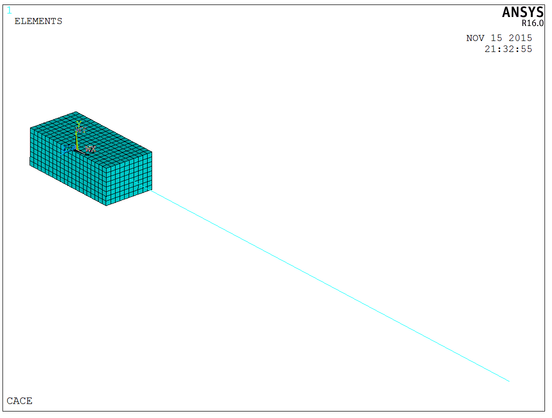
Now, we analyze a specific problem, the model is as shown in the following figure,

For this model, although node 5 is a shared node, the bending moments at the ends do not couple well with the solid element’s bending moment. Therefore, it is necessary to manually create constraint equations. Assuming the solid element is divided into four parts, with node numbers on the connecting surface as shown above, three constraint equations are defined for this model to control the DOFs in three directions. Below is an example of a ROTz constraint equation for node 5,
\[\frac{UX_2 – UX_1d}{Dy_{2 – 1}} = – ROTz_5\]This equation defines the ROTz degree of freedom for node 5 based on the ratio of the difference in horizontal (X direction) and vertical displacements (Y direction) between nodes 1 and 2. Thus, the constraint equation can be rewritten in standard form and represented in ANSYS APDL as,
\[0 = U{X_2} – U{X_1} + ROT{z_5} \times Dy_{2 – 1}\]1 | |
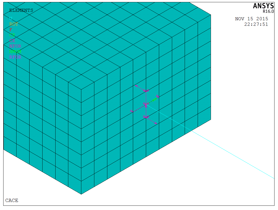
In practical models, if specific node numbers are unknown, the NNEAR command can be used to obtain the nearest node. The finite element model is shown in the following figure,
After building the model, we can define the relevant node constraint equations, three directional constraint equations at the central node are defined in the model with the method described above. The constraints are shown in the following figure,
After applying loading and solving the model, it is clearly shown that the model with defined constraint equations works normally. The following figure shows the bending moment diagram of the beam which is consistent with theoretical analysis,
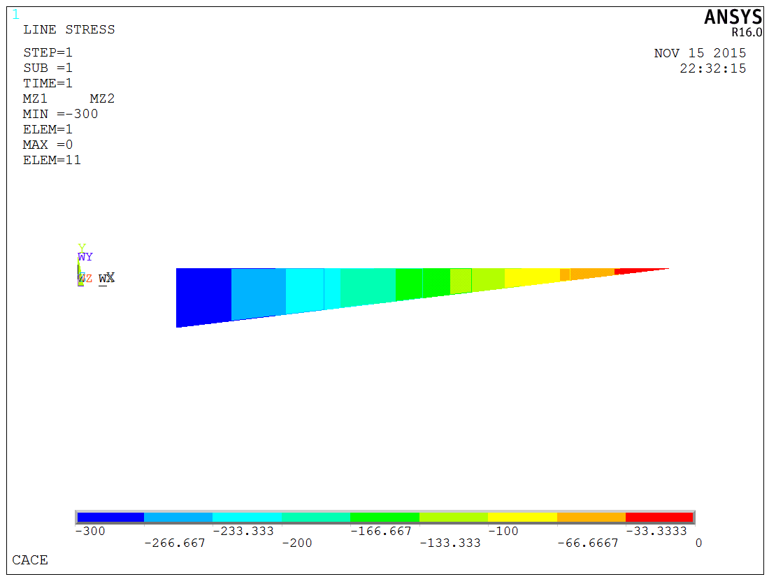
The model is a test model, and the APDL code is available upon request.