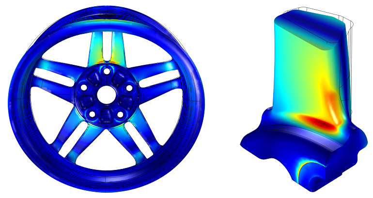
 When finite element models are large, analysis on a standard computer can become challenging. Typically, the model is divided into coarser meshes in such cases, but this comes at the cost of losing analysis precision. When accurate local results are needed for a model’s specific area, the options are either to refine the mesh locally or to use submodel analysis techniques. The former has a significant drawback, mainly because even coarsely divided large models require considerable computational effort. Refining the mesh locally undoubtedly increases the computational load.
Submodel analysis, on the other hand, involves cutting and extracting a local model area, redefining and dividing a finer mesh, applying the actual external loads and boundary conditions on the model, and imposing the original model’s displacement and load conditions forcefully onto the local model basis. This approach allows for obtaining more detailed local results. Submodel analysis ensures the displacement at the cut boundaries of the submodel and the original model is consistent.
According to Ansys Help, submodel analysis has two limitations:
- It is only effective for solid and shell elements.
- The boundaries of the submodel must be far from stress concentration areas.
Submodel analysis in Ansys typically involves the following steps:
- Create the original model and divide it into coarser meshes.
- Create a submodel, divide it into finer meshes, and save the nodes at the boundaries.
- Generate boundary conditions for the submodel based on interpolations from the original model.
- Import the corresponding boundary conditions into the submodel, set the respective loads, and conduct the analysis.
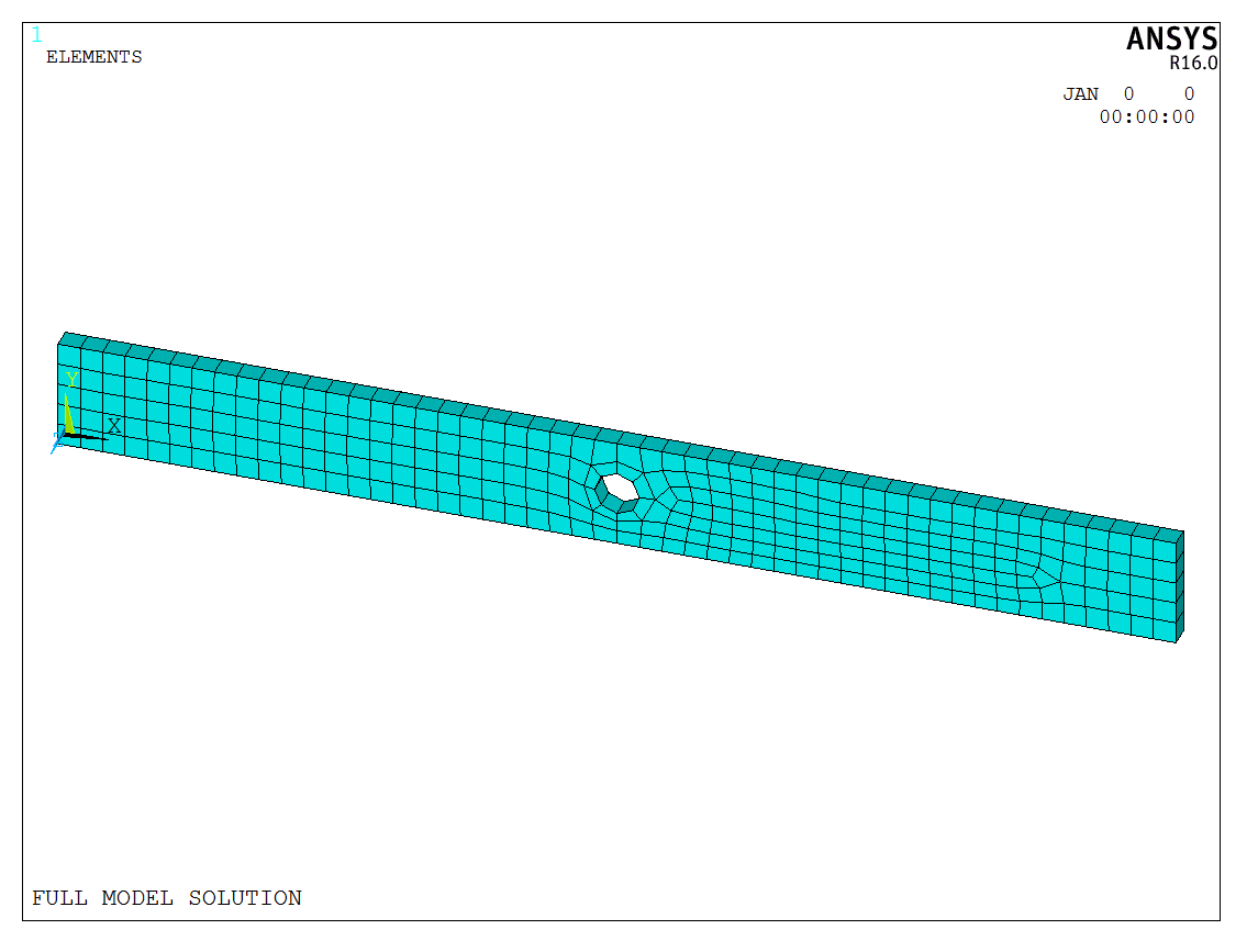
Here is an analysis of a simple example, with the original model as follows,
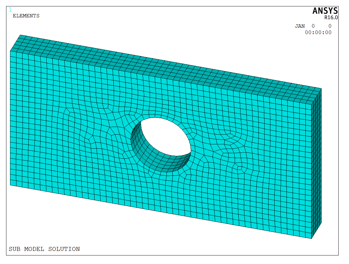
After cutting the model, it is important to note that one can save the original model and then rebuild it, or use /FILNAME to change the file name and save as a new file. The submodel and the original model use the same spatial coordinate system, so the construction position of the submodel is the location of that specific area in the original model. The consistency between the two is crucial because the boundary conditions are generated through spatial coordinate interpolation. The submodel is shown as below,
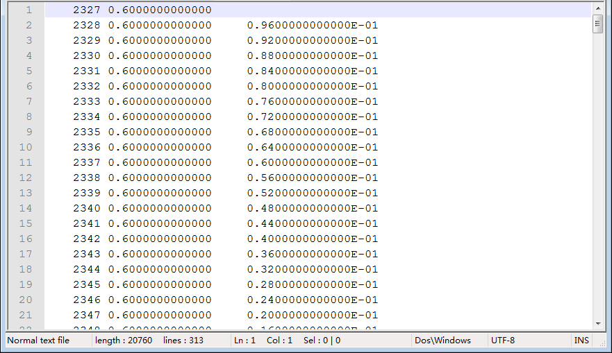
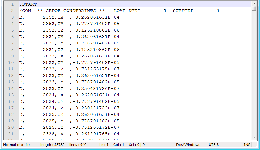
After saving the boundary node data of the submodel, the following file is formed,
In the post-processing /POST1, reopen the original model’s result file and generate boundary condition data using the CBDOF command or through GUI operations,
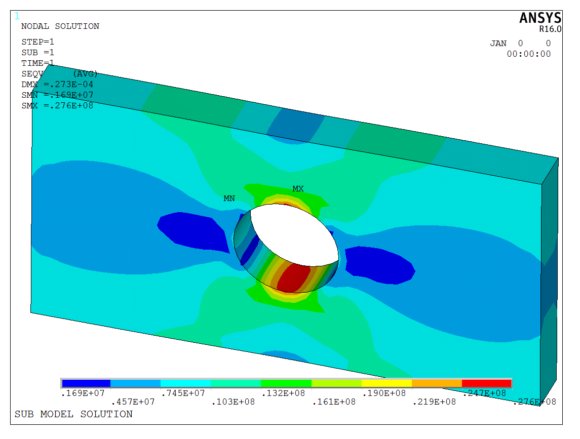
The generated data file is essentially Ansys’s displacement APDL command. Thus, by using /INPUT or GUI to read in the submodel, boundary adjustments can be made, allowing further application of corresponding load conditions and analysis. The final submodel result can be calculated,
The model is a test model, and the APDL code is available upon request.