 In steel structure design, the calculation of component stability is more crucial than the calculation of component strength. Linear buckling analysis tends to be conservative, thus solely conducting a linear eigenvalue analysis is insufficient now. To achieve results closer to real-world engineering scenarios, it is essential to perform nonlinear buckling analysis. In Ansys, the STATIC analysis combined with the application of the arc-length method enables a comprehensive buckling analysis of the component throughout the buckling process.
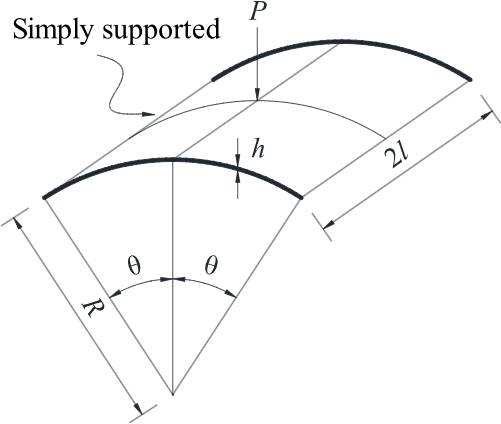
The following image depicts a thin shell with simply supported edges, where the shell radius (R) is 2540mm, length (l) is 254mm, shell thickness (h) is 6.35mm, and arc (θ) is 0.1 rad. The shell experiences a central load of 1000N. This analysis focuses on the elastic shell buckling process.
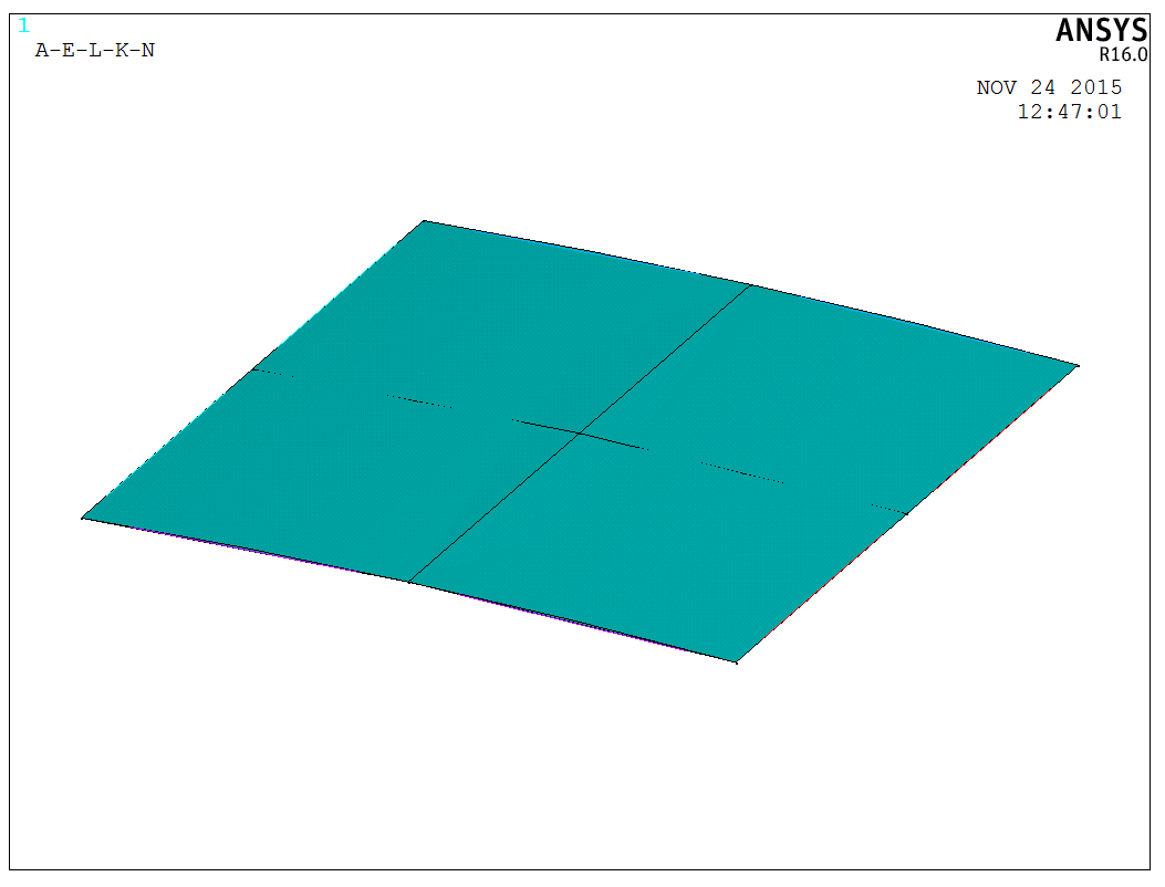
Given the model’s symmetry, it is efficient and adequate to analyze a quarter of the model by adjusting the load to 250N. The finite element model is straightforward to create by change to the cylindrical coordinate system in Ansys, as shown in the figure below:
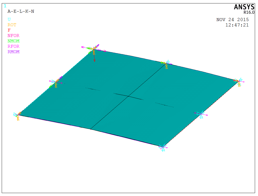
Since the model only represents a quarter-section, the boundary conditions must be adjusted accordingly. Symmetrical boundary conditions are applied along the edges, as well as the concentrated load, as depicted in the following image,
After applying the boundary conditions, we can enter the Solution module. This problem involves nonlinear buckling instability, requiring the activation of the nonlinear calculation option. The arc-length method is used to track the buckling process, with the following considerations:
- Applying a load approximately 10% higher than the estimated load can help identify the buckling load. The estimated load can be obtained from the eigenvalue buckling analysis.
- To enhance computational efficiency, typically two load steps are used here: the first step activates automatic step sizing for the general nonlinear buckling process up to the critical load; the second step activates the arc-length method to proceed through the critical load.
- In the context of arc-length analysis, “Time” refers to the load factor, so its magnitude is arbitrary.
- If convergence issues arise, the NSBSTP in NSUBST command can reduce the initial radius, or the MINARC in ARCLEN command can lower the minimum multiplier of the reference arc-length radius for convergence.
- Use a lower number of equilibrium iterations, generally between 10 to 15.
- To induce the corresponding nonlinear buckling mode, some models may require the application of initial imperfections. Eigenvalue analysis can identify buckling modes, which can then be used to apply geometric imperfections corresponding to those modes for the buckling shape analysis.
With these considerations, we can perform appropriate settings for the arc-length and step size,
1 | |
After the analysis is completed, enter the post-processing module to obtain displacements at different points and the corresponding loads. Here, the load can be calculated by multiplying the time factor “Time” by the total load of 1000N, the following figures show the results at the load point and boundary point, respectively,
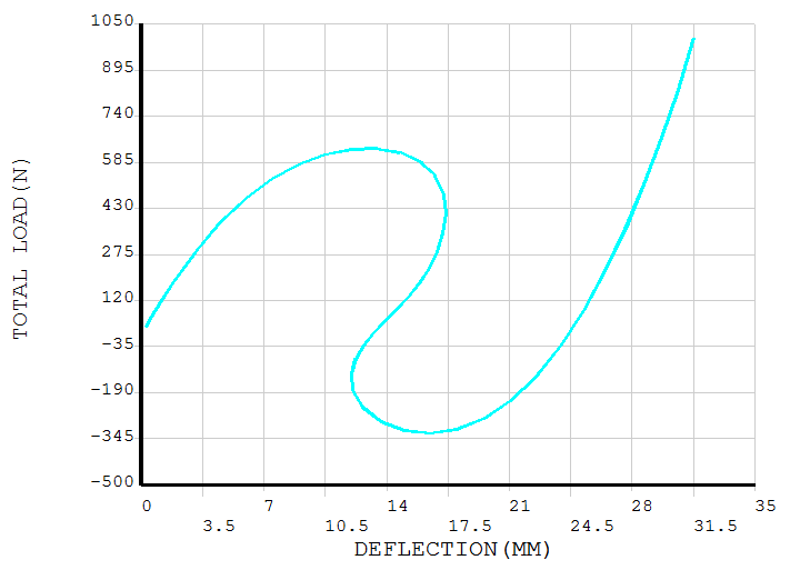
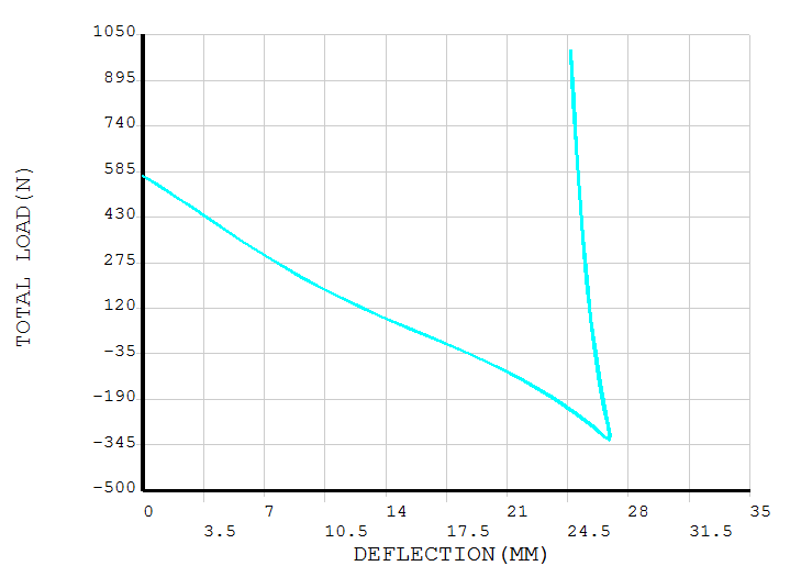
The results demonstrate a significant “snap-through” phenomenon in the shell structure during the buckling process. The image below shows a dynamic Mises stress animation of the complete thin-shell buckling process,
The model is a test model, and the APDL code is available upon request.