 The vector space $ \mathbb{V}$ is introduced in Simple tensor algrbra I, several rules are provided in it. To reduce the abstract, we represent the vectors $ \boldsymbol{x}, \boldsymbol{y}$ with the scalar coefficients $ ({x_1},{x_2},{x_3})$ and $ ({y_1},{y_2},{y_3})$ in $ \mathbb{E}^3$, respectively. The composition of two vectors $ \boldsymbol{x}, \boldsymbol{y} \in\mathbb{E}^3$ is expanded by,
Dot product ($ \cdot $):
\[{\boldsymbol{x}} \cdot {\boldsymbol{y}} = {x_i}{\boldsymbol{g}^i} \cdot {y_j}{\boldsymbol{g}^j} = {x_i}{y_j}{\boldsymbol{g}^i} \cdot {\boldsymbol{g}^j} = {x_i}{y_j}{g^{ij}} = {x^i}{y_i} = \left[ {\begin{array}{cc} {x_1}&{x_2}&{x_3} \end{array}} \right]\left[ {\begin{array}{cc} {y_1}\\ {y_2}\\ {y_3} \end{array}} \right]\]The dot product is also called scalar product or inner product under Cartesian coordinates and it provides the Euclidean magnitudes of these two vectors and the cosine of the angle between them.
Cross product ($ \times$):
\[{\boldsymbol{x}} \times {\boldsymbol{y}} = {x_i}{\boldsymbol{g}^i} \times {y_j}{\boldsymbol{g}^j} = {x_i}{y_j}{\boldsymbol{g}^i} \times {\boldsymbol{g}^j} = {x_i}{y_j}{\varepsilon ^{ijk}}g{\boldsymbol{g}_k} = \left| {\begin{array}{cc} {x_1}&{x_2}&{x_3}\\ {y_1}&{y_2}&{y_3}\\ {\boldsymbol{e}_1}&{\boldsymbol{e}_2}&{\boldsymbol{e}_3} \end{array}} \right|\]The cross product is also called vector product, and it represents the area of a parallelogram with the sides of these two vectors. Now, a new composition for two vectors $ \boldsymbol{x}, \boldsymbol{y} \in\mathbb{E}^3$ is introduced here.
This is not a tutorial, please refer to the books for tensor algebra.
Outer product ($ \otimes $):
\[{\boldsymbol{x}} \otimes {\boldsymbol{y}} = \left[ {\begin{array}{cc} {x_1}\\ {x_2}\\ {x_3} \end{array}} \right]\left[ {\begin{array}{cc} {y_1}&{y_2}&{y_3} \end{array}} \right] = \left[ {\begin{array}{cc} {x_1}{y_1}&{x_1}{y_2}&{x_1}{y_3}\\ {x_2}{y_1}&{x_2}{y_2}&{x_2}{y_3}\\ {x_3}{y_1}&{x_3}{y_2}&{x_3}{y_3} \end{array}} \right]\]Compared with the dot product, it seems we just change the row vector to column vector for $\boldsymbol{x} $ and the column vector to row vector for $ \boldsymbol{y} $. Actually, it is much more complicated than that. The outer product represents the linear mapping from one vector space to another spaces $ \mathbb{V} \to \mathbb{W}$, this linear mapping is also called tensor product.
Linear mapping:
Let $ \mathbb{V}$ and $ \mathbb{W}$ be two vector spaces over the field $ \mathbb{K}$, then if operation $ f: \mathbb{V} \to \mathbb{W}$ satisfies the following two conditions for any $ \boldsymbol{a} \in \mathbb{V}, \boldsymbol{b} \in \mathbb{W}$ and any scalar $ c \in \mathbb{K}$,
- Additivity: $ f(\boldsymbol{a}+\boldsymbol{b}) = f(\boldsymbol{a})+f(\boldsymbol{b})$,
- Homogeneity: $ f(c \boldsymbol{a}) = c f(\boldsymbol{a})$.
is called a linear mapping ($ f \in \textbf{Lin}^n$).
An invertible linear mapping is called an isomorphism.
To be specific, let $ \boldsymbol{w},\boldsymbol{x},\boldsymbol{y} \in \mathbb{E}^3$ be a vector, consider the vector product,
\[\displaystyle \boldsymbol{y}=\underbrace{\boldsymbol{w} \times}_{f} (\boldsymbol{x}) =\hat{\boldsymbol{w}} \boldsymbol{x}= f(\boldsymbol{x})\]the component $ \boldsymbol{w} \times$ can be treated as a linear mapping $ \boldsymbol{x} \to \boldsymbol{y}$. Thus, we use a new symbol $ \hat{\boldsymbol{w}}$ here.
Tensor product:
Go back to the tensor product or outer product, we start from an example.
Example: Consider the projection of a vector $ \boldsymbol{p} \in \mathbb{E}^n$ to another vector $ \boldsymbol{r} \in \mathbb{E}^n$ in the direction of $x \boldsymbol{n} \in \mathbb{E}^n$, this operation can be written by, \(\displaystyle \underbrace{ \boldsymbol{r}}_{\text{result}} =\underbrace{ (\boldsymbol{p} \cdot \boldsymbol{n})}_{\text{coefficient}} \boldsymbol{n} = \underbrace{\boldsymbol{n} (\boldsymbol{n} \cdot }_{\text{map}} \boldsymbol{p})\) note that the RHS is attributed to that the $ \boldsymbol{p} \cdot \boldsymbol{n}$ is a scalar and the dot product satisfies the commutativity. Such operation can be verified with the linear mapping condition and be denoted by, \(\displaystyle \boldsymbol{r} = \boldsymbol{n}( \boldsymbol{n} \cdot \boldsymbol{p}) = (\boldsymbol{n} \otimes \boldsymbol{n}) \boldsymbol{p}\) The $ \otimes $ operation here is actually the same with preceding one in outer product section.
Now, let $ \boldsymbol{a}$ and $ \boldsymbol{b}$ be two vectors in $ \mathbb{E}^n$, an arbitary vector $ \boldsymbol{x}$ can be mapped into the vector space $ \boldsymbol{a} (\boldsymbol{b} \cdot \boldsymbol{x}) $, the mapping operation is denoted by $\boldsymbol{a} \otimes \boldsymbol{b}$. Then,
\[\displaystyle \boldsymbol{a} (\boldsymbol{b} \cdot \boldsymbol{x}) = (\boldsymbol{a} \otimes \boldsymbol{b}) \boldsymbol{x} = (\boldsymbol{x} \cdot \boldsymbol{b}) \boldsymbol{a} = \boldsymbol{x} (\boldsymbol{b} \otimes \boldsymbol{a})\]Tensor product properties:
Linear mapping:
\[\displaystyle (\boldsymbol{a} \otimes \boldsymbol{b}) (\boldsymbol{x}+\boldsymbol{y}) = (\boldsymbol{a} \otimes \boldsymbol{b}) \boldsymbol{x}+(\boldsymbol{a} \otimes \boldsymbol{b}) \boldsymbol{y}, \forall \boldsymbol{x},\boldsymbol{y} \in \mathbb{E}^n\] \[\displaystyle (\boldsymbol{a} \otimes \boldsymbol{b}) (c \boldsymbol{x}) = c(\boldsymbol{a} \otimes \boldsymbol{b}) \boldsymbol{x}, \forall \boldsymbol{x},\boldsymbol{y} \in \mathbb{E}^n, c \in \mathbb{R}\]Associativity:
\[\displaystyle (\boldsymbol{a} \otimes \boldsymbol{b})\otimes \boldsymbol{c} = \boldsymbol{a} \otimes (\boldsymbol{b} \otimes \boldsymbol{c})=\boldsymbol{a} \otimes \boldsymbol{b} \otimes \boldsymbol{c}\] \[\displaystyle c(\boldsymbol{a} \otimes \boldsymbol{b}) = (c \boldsymbol{a}) \otimes \boldsymbol{b} = \boldsymbol{a} \otimes (c \boldsymbol{b}) = c\boldsymbol{a} \otimes \boldsymbol{b}\] \[\displaystyle (c\boldsymbol{a}) \otimes (d\boldsymbol{b}) = (cd)( \boldsymbol{a} \otimes \boldsymbol{b})\]Distributivity:
\[\displaystyle \boldsymbol{a} \otimes (\boldsymbol{b} + \boldsymbol{c})= \boldsymbol{a} \otimes \boldsymbol{b} + \boldsymbol{a} \otimes \boldsymbol{c}\] \[\displaystyle (\boldsymbol{a} + \boldsymbol{b}) \otimes \boldsymbol{c}= \boldsymbol{a} \otimes \boldsymbol{c} + \boldsymbol{b} \otimes \boldsymbol{c}\] \[\displaystyle (\boldsymbol{a} + \boldsymbol{b}) \otimes (\boldsymbol{c} + \boldsymbol{d}) = \boldsymbol{a}\boldsymbol{c}+\boldsymbol{a}\boldsymbol{d}+\boldsymbol{b}\boldsymbol{c}+\boldsymbol{b}\boldsymbol{d}\]Note that the commutativity is not satisfied any more:
\[\displaystyle \boldsymbol{a} \otimes \boldsymbol{b} \ne \boldsymbol{b} \otimes \boldsymbol{a}\]we will prove that the transpose of $ \boldsymbol{a} \otimes \boldsymbol{b}$ is $ \boldsymbol{b} \otimes \boldsymbol{a}$ later.
Example: Proof the distributivity $ \boldsymbol{a} \otimes (\boldsymbol{b} + \boldsymbol{c})= \boldsymbol{a} \otimes \boldsymbol{b} + \boldsymbol{a} \otimes \boldsymbol{c}$ Consider the definition of tensor product, we select a vector $\boldsymbol{x} \in \mathbb{E}^n$. Multiplying both sides of the equation by $\boldsymbol{x}$, the LHS can be written by, \(\displaystyle \boldsymbol{a} \otimes (\boldsymbol{b} + \boldsymbol{c}) \boldsymbol{x} = \boldsymbol{a} ((\boldsymbol{b} + \boldsymbol{c}) \cdot \boldsymbol{x}) = \boldsymbol{a} (\underbrace{\boldsymbol{b} \cdot \boldsymbol{x}}_{\text{scalar}} + \underbrace{\boldsymbol{c} \cdot \boldsymbol{x}}_{\text{scalar}}) = \boldsymbol{a} (\boldsymbol{b} \cdot \boldsymbol{x}) + \boldsymbol{a} (\boldsymbol{c} \cdot \boldsymbol{x})\) The RHS can be written by, \(\displaystyle (\boldsymbol{a} \otimes \boldsymbol{b} + \boldsymbol{a} \otimes \boldsymbol{c}) \boldsymbol{x} = (\boldsymbol{a} \otimes \boldsymbol{b})\boldsymbol{x} + (\boldsymbol{a} \otimes \boldsymbol{c}) \boldsymbol{x} = \boldsymbol{a} (\boldsymbol{b}\cdot \boldsymbol{x}) + \boldsymbol{a} (\boldsymbol{c} \cdot \boldsymbol{x})\) Thus, we get the result.
Contraction:
In tensor product, the dot product and the double dot product are usually called the contraction. Let $\boldsymbol{a} \otimes \boldsymbol{b} \otimes \boldsymbol{c} \otimes \boldsymbol{d}$ be a fourth order tensor (we will find that the tensor product yields the high order tensor later), then the dot product contraction are,
\[\displaystyle \boldsymbol{a} \cdot \boldsymbol{b} \otimes \boldsymbol{c} \otimes \boldsymbol{d}= (\boldsymbol{a} \cdot \boldsymbol{b}) \boldsymbol{c} \otimes \boldsymbol{d}\] \[\displaystyle \boldsymbol{a} \otimes \boldsymbol{b} \cdot \boldsymbol{c} \otimes \boldsymbol{d}= (\boldsymbol{b} \cdot \boldsymbol{c}) \boldsymbol{a} \otimes \boldsymbol{d}\] \[\displaystyle \boldsymbol{a} \otimes \boldsymbol{b} \otimes \boldsymbol{c} \cdot \boldsymbol{d}= (\boldsymbol{c} \cdot \boldsymbol{d}) \boldsymbol{a} \otimes \boldsymbol{b}\]The double dot product contraction is the operation that combines four nearby vector under tensor product,
\[\displaystyle \boldsymbol{a} \otimes \boldsymbol{b} : \boldsymbol{c} \otimes \boldsymbol{d}= (\boldsymbol{a} \cdot \boldsymbol{c}) ( \boldsymbol{b} \cdot\boldsymbol{d})\] \[\displaystyle \boldsymbol{a} \otimes \boldsymbol{b} \cdot \cdot \boldsymbol{c} \otimes \boldsymbol{d}= (\boldsymbol{a} \cdot \boldsymbol{d}) ( \boldsymbol{b} \cdot\boldsymbol{c})\]Rotation:
The rotation operation of a vector is a typical example to show the usage of vector product. In continuum mechanics, the rotation matrix and the transformation matrix are very useful to compute the stress and strain tensor in different orientations. The rotation matrix can be constructed by a rotation axis vector $ \boldsymbol{p}$ (unit vector) and a rotation angle $ \alpha$, we assume the rotation follows the right-hand rule. The result can be written by,
\[\displaystyle {\bf R} = \cos \alpha \; {\bf I} + (1 - \cos \alpha) {\boldsymbol p} \otimes {\boldsymbol p} - \sin \alpha \; {\hat {\boldsymbol p}} \qquad (1)\]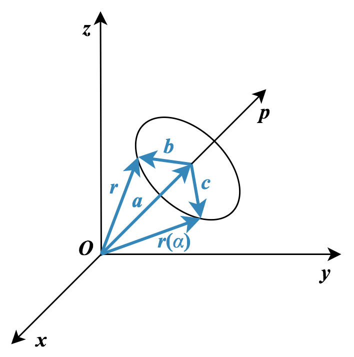
To get such result, we first construct a local coordinate system. Denote $ \boldsymbol x,\boldsymbol y,\boldsymbol z$ are the bases of the Cartesian coordinate system as shown in the figure. $ \boldsymbol g_1$ is a unit vector that aligns with vector $ \boldsymbol b$, $\boldsymbol g_3 $ is a unit vector that aligns with vector $ \boldsymbol p$. Then, the last unit vector can be expressed by $\boldsymbol g_2 = \boldsymbol g_3 \times \boldsymbol g_1$. The position of vector $\boldsymbol r$ rotates to the position $ \boldsymbol r(\alpha)$ with a rotation angle $ \alpha$ about the axis $ \boldsymbol p$. First, the vector $ \boldsymbol r$ can be written by,
\[\displaystyle \boldsymbol r =\boldsymbol a +\boldsymbol b =|\boldsymbol a| \boldsymbol g_3 +|\boldsymbol b| \boldsymbol g_1 \qquad (2)\]Then, after the rotation,
\[\displaystyle \boldsymbol r(\alpha) =\boldsymbol a +\boldsymbol c =|\boldsymbol a| \boldsymbol g_3 +\boldsymbol c \qquad (3)\]Since the length of vector $ \boldsymbol c $ is the same as $ \boldsymbol b $, expand the vector $ \boldsymbol c$ in local coordinate system,
\[\displaystyle \boldsymbol c = |\boldsymbol b| \cos(\alpha) \boldsymbol g_1 + |\boldsymbol b| \sin(\alpha) \boldsymbol g_2 \qquad (4)\]Thus,
\[\displaystyle \boldsymbol r(\alpha) =\boldsymbol a +\boldsymbol c =|\boldsymbol a| \boldsymbol g_3 +|\boldsymbol b| \cos(\alpha) \boldsymbol g_1 + |\boldsymbol b| \sin(\alpha) \boldsymbol g_2 \qquad (5)\]Note that we want to construct a mapping operation $ f(\boldsymbol p, \alpha)$ (i.e. $ f(\boldsymbol g_3, \alpha)$) that satisfies $\boldsymbol r(\alpha) = f(\boldsymbol p, \alpha) \boldsymbol r$, so we need to eliminate $ \boldsymbol r$ from the preceding equation $ (5)$ to get $ f(\boldsymbol p, \alpha)$ (i.e. $ f(\boldsymbol g_3, \alpha)$). Consider that the vector $ \boldsymbol a$ is a projection of vector $x \boldsymbol r$ on rotation axis $ \boldsymbol p$, then,
\[\displaystyle \boldsymbol a =|\boldsymbol a| \boldsymbol g_3= (\boldsymbol r \cdot \boldsymbol g_3) \boldsymbol g_3 = \boldsymbol g_3 (\boldsymbol g_3 \cdot \boldsymbol r) = (\boldsymbol g_3 \otimes \boldsymbol g_3) \boldsymbol r \qquad (6)\]and from equation $ (2)$,
\[\displaystyle|\boldsymbol b| \boldsymbol g_1 =\boldsymbol r -|\boldsymbol a| \boldsymbol g_3 \qquad (7)\]Plug $ (6)$ and $ (7)$ into equation $ (5) $ and note that $ \boldsymbol g_2 = \boldsymbol g_3 \times \boldsymbol g_1$,
\[\displaystyle \boldsymbol r(\alpha) = (\boldsymbol g_3 \otimes \boldsymbol g_3) \boldsymbol r + \cos(\alpha) (\boldsymbol r -|\boldsymbol a| \boldsymbol g_3) + |\boldsymbol b| \sin(\alpha) (\boldsymbol g_3 \times \boldsymbol g_1) \qquad (8)\]Rearrange the equation,
\[\displaystyle \boldsymbol r(\alpha) = (\boldsymbol g_3 \otimes \boldsymbol g_3) \boldsymbol r + \cos(\alpha) \boldsymbol r - \cos(\alpha) (\boldsymbol g_3 \otimes \boldsymbol g_3) \boldsymbol r + \sin(\alpha) (\boldsymbol g_3 \times |\boldsymbol b|\boldsymbol g_1) \qquad (9)\]Since $ \boldsymbol r = \lvert \boldsymbol a \rvert \boldsymbol g_3 + \lvert \boldsymbol b\rvert \boldsymbol g_1$, the corss product $ \boldsymbol g_3 \times \lvert \boldsymbol b \rvert \boldsymbol g_1$ can be written by,
\[\displaystyle \boldsymbol g_3 \times |\boldsymbol b|\boldsymbol g_1 =\boldsymbol g_3 \times (\boldsymbol r -|\boldsymbol a| \boldsymbol g_3) =\boldsymbol g_3 \times \boldsymbol r \qquad (10)\]Thus,
\[\displaystyle \boldsymbol r(\alpha) = (\boldsymbol g_3 \otimes \boldsymbol g_3) \boldsymbol r + \cos(\alpha) \boldsymbol r - \cos(\alpha) (\boldsymbol g_3 \otimes \boldsymbol g_3) \boldsymbol r + \sin(\alpha) (\boldsymbol g_3 \times \boldsymbol r) \qquad (11)\] \[\displaystyle \boldsymbol r(\alpha) =[ (\boldsymbol g_3 \otimes \boldsymbol g_3) + \cos(\alpha) \mathbf{I} - \cos(\alpha) (\boldsymbol g_3 \otimes \boldsymbol g_3) + \sin(\alpha) \hat{\boldsymbol g }_3] \boldsymbol r \qquad (12)\] \[\displaystyle \boldsymbol r(\alpha) =[ (\boldsymbol g_3 \otimes \boldsymbol g_3) (1 - \cos(\alpha))+ \cos(\alpha) \mathbf{I} + \sin(\alpha) \hat{\boldsymbol g }_3] \boldsymbol r \qquad (13)\]$ \boldsymbol g_3$ is the vector $ \boldsymbol p$ in equation $ (1)$, thus we get the result.