 During analysis, we often encounters complex boundary conditions that vary with time, coordinates, temperature, and other factors. Therefore, it is not feasible to apply a general loading method to impose loads on structures, such as loads that change with spatial location or convective boundaries in thermal convection analysis that vary with coordinate position.
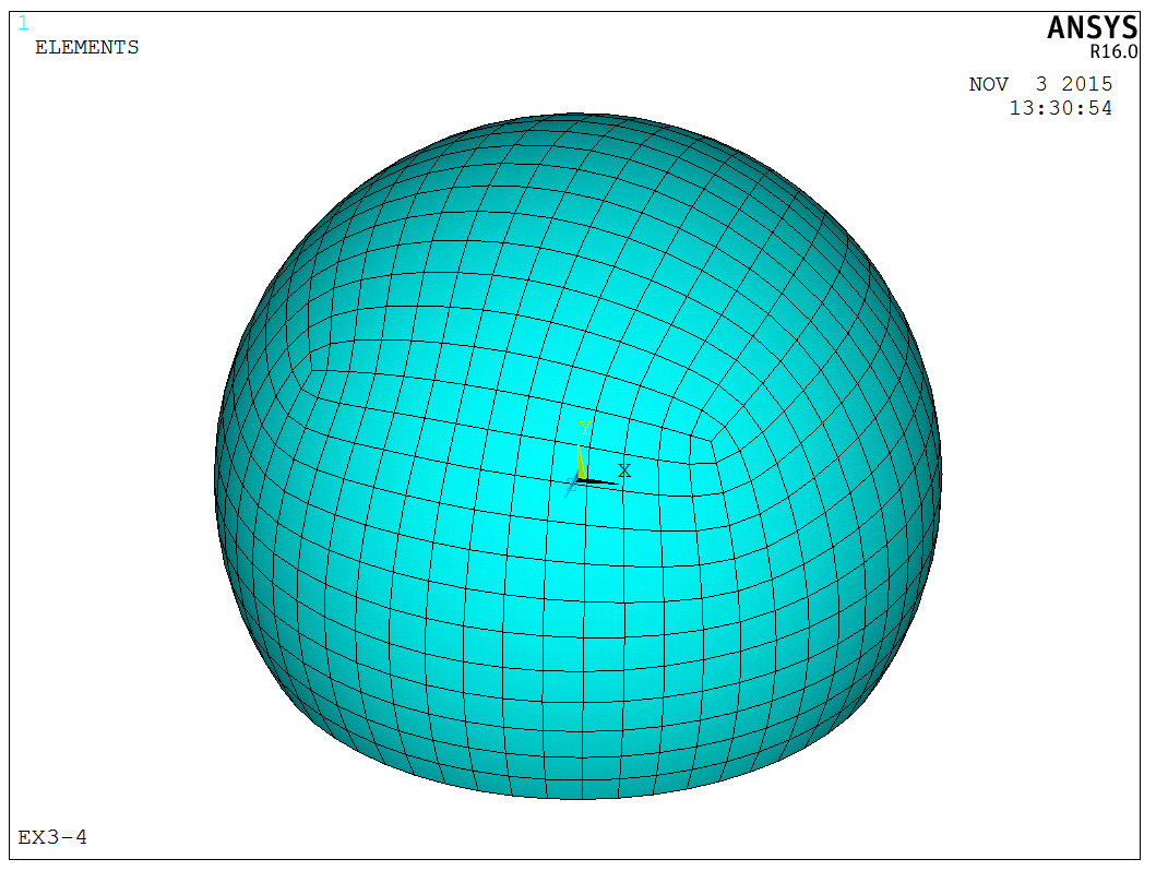
For the application of such complex boundary conditions, function boundary conditions can typically be used. This post analyzes a hollow spherical shell model, which is basically depicted as follows,

The radius of the spherical shell is 7850 mm, with a wall thickness of 44 mm, subjected to a wind load excitation of 60m/s wind speed. The bottom opening is constrained as a simple support. In the analysis, the wind load excitation is simplified into a loading function,
\[P = 0.441 \times \left| {\sin (\omega t)} \right| \times (0.5 \times {\cos ^2}\phi \times \cos \theta – {\sin ^2}\phi )\]The above load form is given in spherical coordinates, so it is also necessary to add it in the form of spherical coordinates in ANSYS. Below we begin modeling, adopting the strategy of forming surfaces through the rotation of arcs, as shown in the following figure,
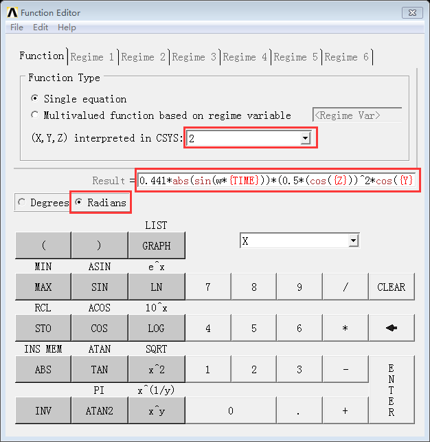
Next, we need to generate the wind speed load. First, the above expression should be converted into ANSYS’s format. In ANSYS, all built-in variables are enclosed in curly braces, such as {TIME} representing time, so the loading function above can be written as,
1 | |
Then, the function editor can be opened, and the above expression can be filled in,
Afterward, one can click GRAPH to set the plot information,
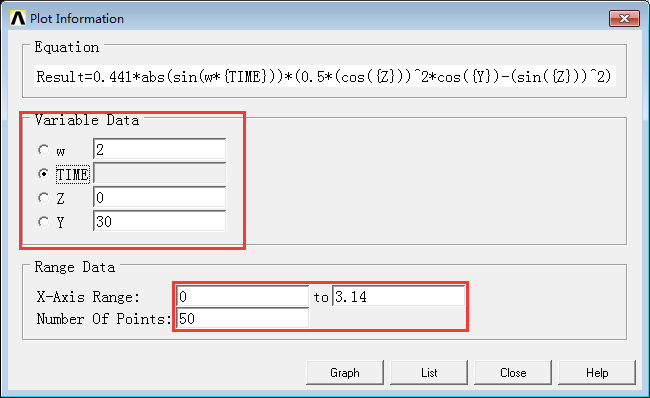
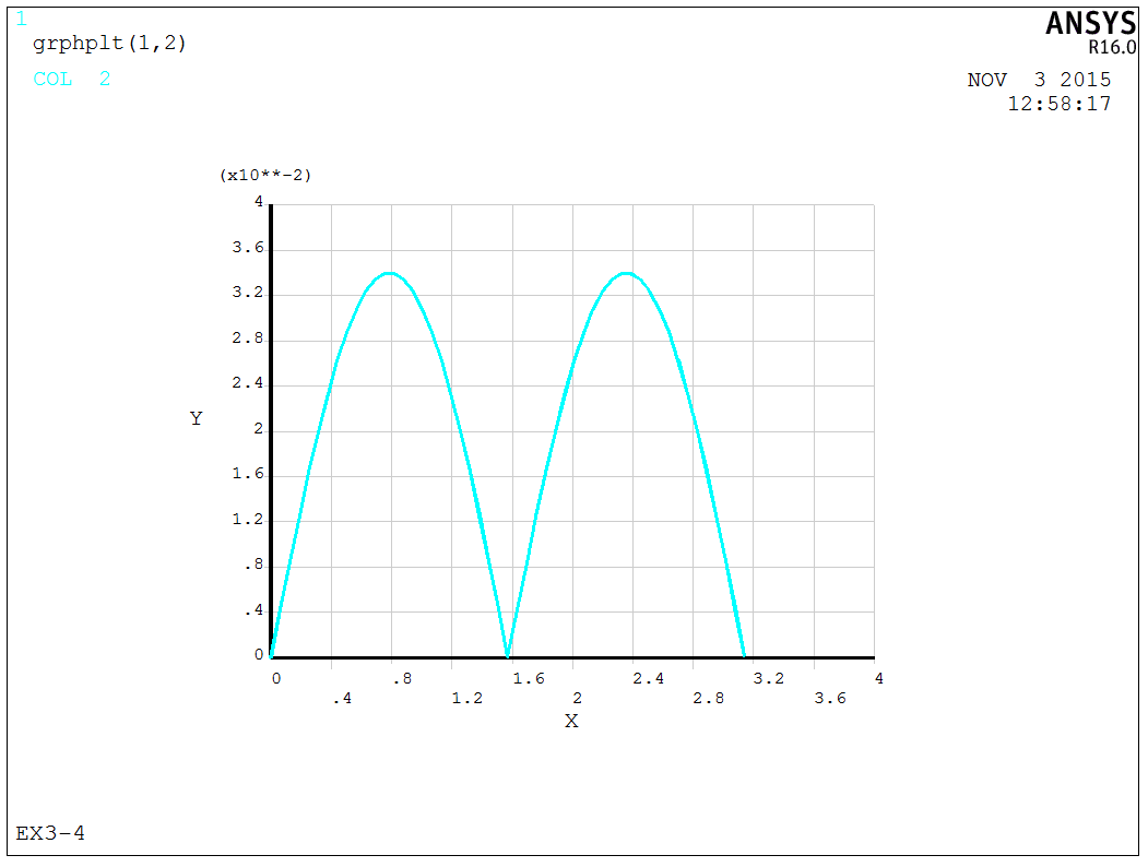
Clicking GRAPH directly can display the load curve,
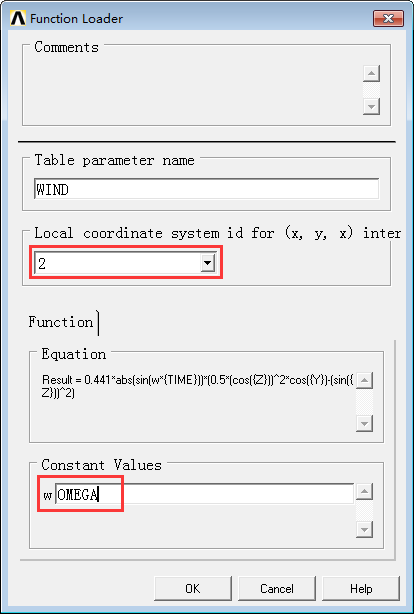
If correct, return to the function editing dialog box and save the function, here we saved it as WIND.func. Then, open the function loader dialog box, select the function file, and load it into TABLE for loading preparation. In the function loader dialog box, the system will ask you to choose the Constant values in the function, here it is the frequency, which can be replaced by a constant or a variable. If replaced by a variable, this variable needs to be defined in advance during the modeling process.
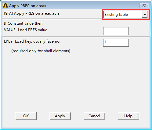
After the function is converted to TABLE, the SFA command can be used to add the TABLE load. During loading, select the Existing table to load the pre-defined TABLE load:
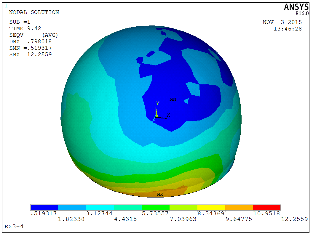
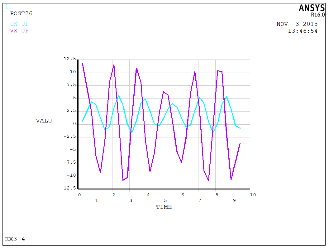
Then, apply the boundary conditions and solve. This post uses transient analysis, and the figure below shows part of the results (Bending moment contour in X direction, Displacement versus time in X direction):
The model is a test model, and the APDL code is available upon request.