 Last time, when solving differential equations with Mathematica built-in solver, I found that while the precision of the solutions was great, the speed left much to be desired. To increase the calculation speed of seismic response spectra and enable the simultaneous computation of spectra under various damping ratios, we need a new method. The standard approach is the Newmark method, but this time, I explored a more conventional recursive algorithm. This method is simple and efficient in computation. Also it can provide displacement, velocity, and acceleration spectra all at once.
Basic knowledge
Structural dynamic responses can be inefficient computed with Duhamel’s integral. Even for simple load types, the complexity can stil increase significantly. Earthquake waves, often irregular, cannot be represented by simple mathematical expressions. Even previous attempts at using interpolation functions were inefficient. Thus, considering practicality, numerical methods for earthquake response calculation are essential.
There are two numerical methods for earthquake response calculation:
- Interpolating method
- Numerical integration
Both methods are suitable for linear systems, but only the second is effective for nonlinear systems.
Time-stepping method
Following structural dynamics book, differential equations can be solved using a time-stepping approach. The basic equation for a single-degree-of-freedom system under earthquake influence is as follows,
\[m\ddot u + c\dot u + ku = p(t)\]or,
\[m\ddot u + c\dot u + ku = – m{u_g}(t)\]With initial conditions,
\[\begin{array}{l} \dot u(0) = 0\\ u(0) = 0 \end{array}\]At time $i$, the dynamic equation becomes,
\[m{\ddot u}_i + c{\dot u}_i + k{u_i} = {p_i}\]The challenge is to find a recursive method that accurately calculates displacement, velocity, and acceleration for time $i+1$ based on these conditions, effective for all $i=0,1,2…$,
\[{m{\ddot u}_{i + 1} + c{\dot u}_{i + 1} + k{u_{i + 1}} = {p_{i + 1}}}\]Such a method would be a viable means to compute response spectra.
External load interpolation
Assuming the external load at time $i$ is $F_i$, the force $F(\tau)$ between $\tau$ and $(i < \tau \le i + 1)$ can be,
\[F\left( \tau \right) = {F_i} + \left( {\frac{\Delta {F_i}}{\Delta t}} \right)\tau\]where,
\[\begin{array}{l} \Delta {F_i} = {F_{i + 1}} – {F_i}\\ \Delta t = {t_{i + 1}} – {t_i} \end{array}\]Thus, $F(\tau)$ is the interpolated force between $0$ and $\Delta t$.
For the motion equation for an undamped single-degree-of-freedom system, the equation can be given by,
\[\ddot u + \omega _n^2u = \frac{1}{m}\left[ {F_i + \left( {\frac{\Delta {F_i}}{\Delta t}} \right)\tau } \right]\]The above equation can be resolved by superimposing the general solution and the special solution. The general solution is the solution for ${u_i}$ and ${\dot u}_i$ at $\tau =0$. The special solution can be decomposed into,
- Response from ${F_i}$
- Response from $\left( {\frac{\Delta {F_i}}{\Delta t}} \right)\tau$
Thus, we can get,
\[{u_{i + 1}} = {u_i}\cos ({\omega _n}\Delta t) + \left( {\frac{\dot u_i}{\omega_n}} \right)\sin ({\omega _n}\Delta t) + \frac{F_i}{k}\left[ {1 – \cos ({\omega _n}\Delta t)} \right] + \\ \left( {\frac{\Delta {F_i}}{k}} \right)\left( {\frac{1}{\omega_n \Delta t}} \right)\left[ {\omega_n \Delta t – \sin \left( {\omega_n \Delta t} \right)} \right]\] \[\frac{\dot u_{i + 1}}{\omega_n} = – {u_i}\sin ({\omega _n}\Delta t) + \left( {\frac{\dot u_i}{\omega_n}} \right)\cos ({\omega _n}\Delta t) + \frac{F_i}{k}\sin ({\omega _n}\Delta t) + \\ \left( {\frac{\Delta {F_i}}{k}} \right)\left[ {1 – \cos \left( {\omega_n \Delta t} \right)/{\omega _n}\Delta t} \right]\]The recursive equation for a damping system can be calculated in the same way. The following will be expressed in a simpler way,
\[\begin{array}{l} {u_{i + 1}} = a{u_i} + b{\dot u}_i + c{F_i} + d{F_{i + 1}}\\ {\dot u}_{i + 1} = {a_1}{u_i} + {b_1}{\dot u}_i + {c_1}{F_i} + {d_1}{F_{i + 1}} \end{array}\]where,
\[a = {e^{ – \rho {\omega _n}\Delta t}}\left( {\rho \sin {\omega _d}\Delta t + \sqrt {1 – {\rho ^2}} \cos {\omega _d}\Delta t} \right)/\sqrt {\left( {1 – {\rho ^2}} \right)}\] \[b = {e^{ – \rho {\omega _n}\Delta t}}\left( {\frac{1}{\omega_d}\sin {\omega _d}\Delta t} \right)\] \[c = \frac{1}{k{\omega_n}\Delta t}\left\{ {2\rho + {e^{ – \rho {\omega _n}\Delta t}}{\omega _n}\Delta t\kappa } \right\}\] \[\kappa {\rm{ = }}\left[ {\left( {\frac{1 – 2{\rho ^2}}{\omega_d \Delta t} – \frac{\rho }{\sqrt {1 – {\rho ^2}} }} \right)\sin {\omega _d}\Delta t – \left( {1 + \frac{2\rho }{\omega_n \Delta t}} \right)\cos {\omega _d}\Delta t} \right]\] \[d = \frac{1}{k{\omega _n}\Delta t}\left\{ {\omega_n \Delta t – 2\rho + {e^{ – \rho {\omega _n}\Delta t}}{\omega_n} \Delta t \alpha} \right\}\] \[\alpha = \left[ {\left( {\frac{2{\rho ^2} – 1}{\omega_d \Delta t}} \right)\sin {\omega _d}\Delta t + \left( {\frac{2\rho }{\omega_n \Delta t}} \right)\cos {\omega _d}\Delta t} \right]\] \[{a_1} = – {e^{ – \rho {\omega _n}\Delta t}}\left( {\frac{\omega_n}{\sqrt {1 – {\rho ^2}} }\sin {\omega _d}\Delta t} \right)\] \[{b_1} = – {e^{ – \rho {\omega _n}\Delta t}}\left( { – \rho \sin {\omega _d}\Delta t + \sqrt {1 – {\rho ^2}} \cos {\omega _d}\Delta t} \right)/\sqrt {\left( {1 – {\rho ^2}} \right)}\] \[{c_1} = \frac{1}{k\Delta t}\left\{ { – 1 + {e^{ – \rho {\omega _n}\Delta t}}\left[ {\left( {\frac{\omega_n \Delta t}{\sqrt {1 – {\rho ^2}} } + \frac{\rho }{\sqrt {1 – {\rho ^2}} }} \right)\sin {\omega _d}\Delta t + \cos {\omega _d}\Delta t} \right]} \right\}\] \[{d_1} = \frac{1}{k\Delta t}\left\{ {1 – {e^{ – \rho {\omega _n}\Delta t}}\left[ {\frac{\rho }{\sqrt {1 – {\rho ^2}} }\sin {\omega _d}\Delta t + \cos {\omega _d}\Delta t} \right]} \right\}\]This leads to a recursive expression for damped systems. By starting with zero initial displacement and velocity, displacement and velocity at any moment can be calculated.
Implementing Response Spectra Calculation in MMA
With initial displacement and velocity as starting values, displacement and velocity curves can be computed. Extracting maximum values and storing them in arrays allows for the generation of response spectra.
After importing the earthquake wave and initializing arrays for displacement, velocity, and acceleration, extract the wave length and time interval,
1 | |
We need to convert the earthquake wave to the SI unit system, initialize damping, and sampling interval, then prepare arrays for maximum displacement, velocity, and acceleration values based on the sampling number. For instance, sampling 200 times at 0.05s intervals means calculating for a period range of 0-10s, this can obtain maximum values for each displacement, velocity, and acceleration curve every 0.05s,
1 | |
The main loop involves a complete time history calculation for each damping ratio and sampling point. We need to repeat 1200 times in total to calculate displacement, velocity, and acceleration for every point (1560 points in total) of the Elcentro earthquake wave for 6 different damping ratios,
1 | |
After calculating the response spectra values, they can be plotted with the following command. It should be noted that display positions might vary across different computers,
1 | |
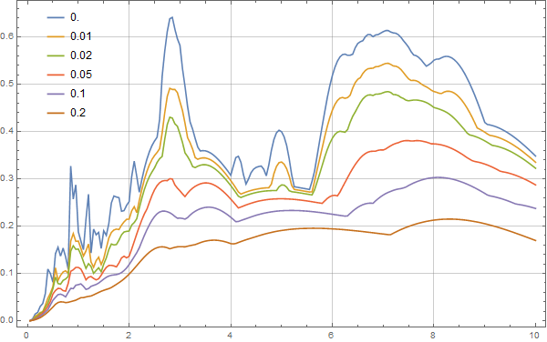
The resulting displacement spectrum is shown below,
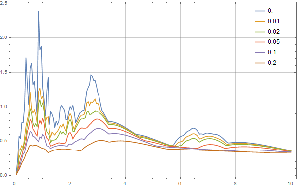
The velocity spectrum is as follows,
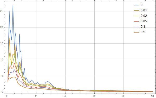
The acceleration spectrum appears as,
Efficiency Comparison with MATLAB
Aside from the plotting function, the program does not rely heavily on advanced functions specific to mathematical software. A calculation in MATLAB shows that processing five earthquake waves took approximately 19s in Mathematica but only about 13s in MATLAB. A closer examination revealed that Mathematica recursive calculations at the loop end were notably slower, indicating its unsuitability for intensive matrix computations.
Conclusion
This recursive calculation method is straightforward, brute-force, and effective. I think it is the most convenient method for computing response spectra. With a basic understanding of the algorithm, we can develop a respectable software for calculating response spectra, whether in C++ or Python.
The full script can be downloaded here: DOWNLOAD