Mathematica seismic response spectrum

Previously, I calculated the velocity and displacement time histories of an earthquake wave based on its acceleration. I want to know whether it was possible to directly compute the response spectrum of the earthquake wave. Given that Mathematica comes equipped with a differential equation solver, solving second-order differential equations without having to write code manually is much more convenient. Therefore, this post will utilize Mathematica NDSolveValue to calculate the response spectrum of an earthquake wave.

Fundamental knowledge

The general response spectrum is intended for a fixed damping ratio, so different response spectra can be obtained for different damping ratios. In practice, spectra from multiple damping values are combined for use. This can cover the damping characteristics of various actual structures. When calculating the response spectrum, choosing frequency or period as the independent variable is arbitrary. Typically, the period is the more common choice, and standards also use the period as the independent variable.

There are many types of response spectra, with displacement, velocity, and acceleration spectra being the most commonly used in structural dynamics:

\[\begin{array}{l} {u_0}({T_n},\varsigma ) = \mathop {\max }\limits_t \left| {u(t,{T_n},\varsigma )} \right|\\ {\dot u_0}({T_n},\varsigma ) = \mathop {\max }\limits_t \left| {\dot u(t,{T_n},\varsigma )} \right|\\ {\ddot u_0}({T_n},\varsigma ) = \mathop {\max }\limits_t \left| {\ddot u(t,{T_n},\varsigma )} \right| \end{array}\]

In this post, we will calculate a displacement spectrum for an earthquake wave, using the period as the independent variable.

Calculation process

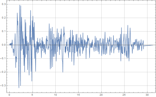
First, we need to obtain an earthquake wave. We will use the El Centro wave, which can be downloaded from vibrationdata. The downloaded wave has already been corrected, so no further processing is needed. This wave is imported into Mathematica,

Clear["Global`*"]
data = Import[NotebookDirectory[] <> "elcentro.dat"];
acc = Interpolation[data]
tmin = (Min /@ Transpose[data])[[1]];
tmax = (Max /@ Transpose[data])[[1]];
Plot[acc[x], {x, tmin, tmax}, PlotRange -> All, Frame -> True, GridLines -> Automatic, ImageSize -> 600]

The processing here is the same as for the previous earthquake wave velocity and displacement time histories. This allow us to directly plot the time history curve of the earthquake wave,

Next, we set some basic parameters for the single-degree-of-freedom system to be excited,

dampRatio = 0.02;
sampleTime = 10;
samplePoint = 10;
eigenPeriod = Table[i, {i, sampleTime/samplePoint, sampleTime, sampleTime/samplePoint}];
dispSet = Table[0, {samplePoint}];

We set the damping ratio to 0.02 and the calculation period to 10s, with 10 sampling points for the calculation. It is important to initialize the variable for storing peak displacement to avoid errors later on.

After importing the earthquake wave for plotting, we have obtained the acceleration interpolation function acc. Thus, acc[t] represents the ground acceleration value at time t. Based on the basic equations of dynamics,

\[\ddot u + 2\varsigma {\omega _n}\dot u + \omega _n^2u = - {\ddot u_g}(t)\]

The earthquake acceleration on the right side of the equation is our obtained function acc[t], which can be directly used, allowing Mathematica to automatically calculate. By combining this with a For loop, we calculate the peak values over ten cycles,

For[i = 1, i <= samplePoint, i++,
    disp = NDSolveValue[{u''[t] + 2*dampRatio*(2*Pi/eigenPeriod[[i]])*u'[t] + (2*Pi/eigenPeriod[[i]])^2*u[t] == -9.8*acc[t], u'[0] == 0, u[0] == 0}, u, {t, tmin, tmax}] ;
    dispSet[[i]] = Max[Abs[Table[disp[x], {x, tmin, tmax, (tmax - tmin)/Length[data]}]]];
]
points = Transpose[{eigenPeriod, dispSet}];
ListLinePlot[points, PlotRange -> All, Frame -> True, GridLines -> Automatic, ImageSize -> 600]

Now, we obtain a simple displacement spectrum,

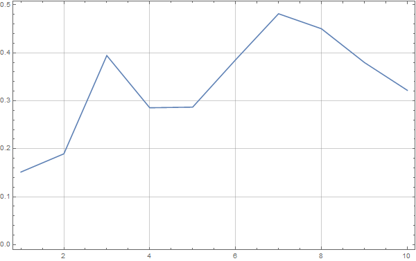
Of course, this spectrum is quite rough, and its detail level can be adjusted by changing the sampling values.

Comparison with SeismoSignal

To ensure accuracy in our response spectrum, it is necessary to compare our results with those from standard software. I have uninstalled DPLOT due to compatibility issues and its tendency to hang the system upon exit. Instead, I have used SeismoSignal for comparison.

After importing the data file into SeismoSignal and switching to the Elastic/Inelastic Response Spectra interface, we directly obtain the earthquake wave response spectrum. We then save this spectrum and import it into Mathematica for comparison,

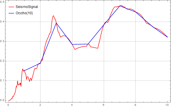
The trends of both are consistent. We then adjust the sampling points to 50, 200, 500, and 1000 for further calculations and comparisons.

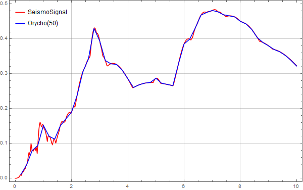
Below are comparison graphs for sampling points of 50,

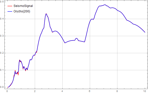
Below are comparison graphs for sampling points of 200,

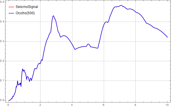
Below are comparison graphs for sampling points of 500,

Below are comparison graphs for sampling points of 1000,

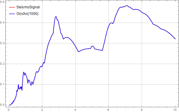
From these images, it is clear that when the sampling points reach 500, the displacement spectrum calculated by MMA matches very well with the data from SeismoSignal.

Limitations and suggestions

Although Mathematica calculation results align closely with those from commonly used software, this method is quite slow. If tried, one will notice that selecting 1000 samples requires a long wait time, significantly longer than with SeismoSignal. SeismoSignal can quickly compute the response spectrum upon acceleration input. Therefore, this method could be improved.

The Newmark method is commonly used for such calculations and is extensively discussed in dynamics textbooks. The method used in this post was chosen for its simplicity and to fully utilize Mathematica capabilities. However, this comes at the cost of significant time consumption.

Conclusion

This algorithm will not be further developed to solve differential equation for speed enhancement. If faster calculations are needed, we can directly use methods from dynamics textbooks.

The full script can be downloaded here: DOWNLOAD