Mathematica seismic wave time history integration

In my previous time history analyses, I utilized SeismoSignal software, a seismic wave processing software developed by SeismoSoft. It allows for filtering, baseline adjustment, and computation of displacement spectra among other features. Considered its capabilities and ease of use, I want to create a similar tool myself.

The tasks included various filtering techniques such as high-pass, low-pass, and band-pass filters; calculation of velocity and displacement time histories; baseline correction; Fourier transform; and computation of velocity and displacement spectra. Initially, the goal was simply to integrate the seismic wave to obtain the velocity and displacement curves. I assumed this to be straightforward, but practical experimentation revealed the complexity of the task. The following just records the analysis process.

Calculation principle

The principle is simple but challenging to implement. Typically, seismic data is provided as acceleration time history curves. Basic physics dictates that by integrating the acceleration curve (assuming an initial velocity of zero), one can obtain the velocity, and a subsequent integration yields the displacement.

While calculating the velocity and displacement values at a specific point is feasible, deriving the entire time history curves is more complex. Beyond the upcoming discussion on baseline correction, extensive integration calculations are required.

\[v(t) = \int_0^t {a(t)dt}\]

For instance, to generate a velocity curve from 2000 acceleration data points, thousands of integrations are necessary, a task that can strain even Mathematica or MATLAB. Rendering a 20-second velocity curve using plotting commands would thus be unfeasible.

1	Plot[NIntegrate[acc[t], {t, 0, x}], {x, 0, 20}]

A new idea in approach is needed here: substituting the integral solver with a differential solver.

In numerical computations, the speed of solving ordinary differential equations (ODEs) is reliably fast. Hence, we solve for the velocity component using the ODE solver.

\[\frac{dv(t)}{dt} = a(t)\]

Velocity time history calculation

Following the analysis, calculations commence with downloading and importing commonly used seismic wave data, such as the Elcentro wave,

1 2 3 4 5 6

Clear["Global`*"] data = Import[NotebookDirectory[] <> "elcentro.dat"]; acc = Interpolation[data]; tmin = (Min /@ Transpose[data])[[1]]; tmax = (Max /@ Transpose[data])[[1]]; Plot[acc[x], {x, tmin, tmax}, PlotRange -> All, Frame -> True, GridLines -> Automatic, ImageSize -> 600]

It should be noted to clear the memory to prevent any other issues. After importing, the seismic wave start and end times (tmin and tmax) are determined, and the acceleration time history curve is plotted here,

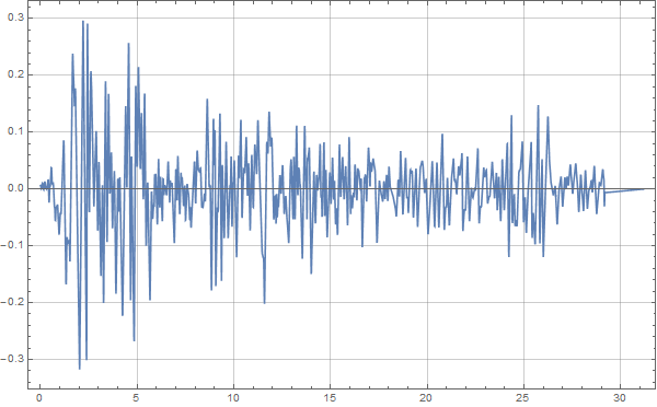
Upon obtaining this data chart, the built-in ODE solver calculates the velocity,

1	velo = NDSolveValue[{velo'[x] == acc[x], velo[0] == 0}, velo, {x, tmin, tmax}];

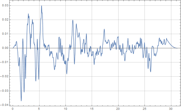
The result, denoted as velo, is plotted to visualize the curve,

It appears satisfactory and meets our requirements.

Baseline correction

After obtaining the velocity curve, an important step is baseline correction. The acceleration data represents only part of the seismic process, and due to sensor sensitivity, data prior to the zero moment is inaccessible. Moreover, sensor inaccuracies can introduce drift. Assuming the ground was stationary before and after the quake (velocity equals zero), we slightly adjust the seismic wave.

Since the seismic wave I downloaded was already corrected, the velocity curve only required minimal adjustment.

A regression calculation based on basic fitting equations yielded a correction function with minor adjustment.

1	velofit = Fit[{{tmin, velo[tmin]}, {tmax, velo[tmax]}}, {1, x, x^2}, x];

\[y = – 2.396 \times {10^{ – 21}} + 3.202 \times {10^{ – 7}}x + 1.027 \times {10^{ – 8}}{x^2}\]

However, to complete the analysis, the velocity curve was recalculated using this method,

1 2	velonew = velo[x] - velofit; Plot[velonew, {x, tmin, tmax}, PlotRange -> All, Frame -> True, GridLines -> Automatic, ImageSize -> 600]

Though the difference appeared minor, the velocity should be corrected anyway,

Displacement time history calculation

Using a similar approach for displacement time history calculation,

1 2	disp = NDSolveValue[{disp'[x] == velonew, disp[0] == 0}, disp, {x, tmin, tmax}]; Plot[disp[x], {x, tmin, tmax}, PlotRange -> All, Frame -> True, GridLines -> Automatic, ImageSize -> 600]

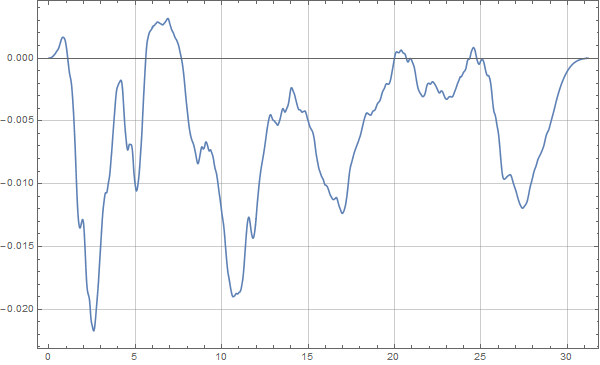
Now, we obtained the Elcentro wave displacement curve,

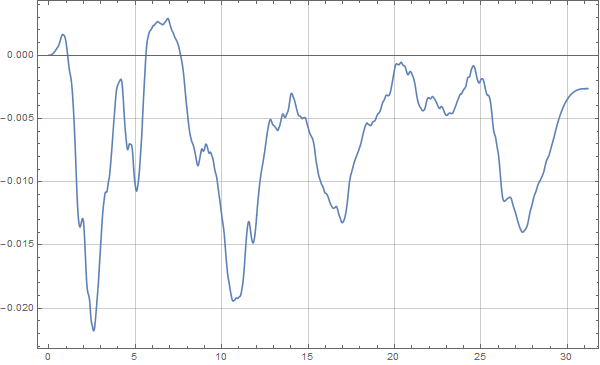
However, a permanent ground displacement was observed post-quake, which, while possible, sometimes requires correction for model analysis. A cubic regression function was set, plotted,

1 2 3 4

trend = disp; fit = Fit[{{tmin, trend[tmin]}, {tmax, trend[tmax]}}, {1, x, x^2, x^3}, x]; removetrend = disp[x] - fit; Plot[{disp[x], fit}, {x, tmin, tmax}, PlotRange -> All, Frame -> True,GridLines -> Automatic, ImageSize -> 600]

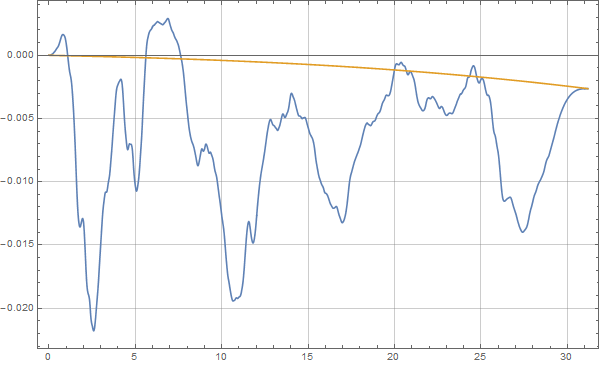
The baseline drift was removed to achieve a drift-free displacement time history,

DPLOT verification

To verify our analysis and calculations, I used DPLOT, a simpler data processing software similar to SeismoSignal. Despite its simplicity, it is not cheap.

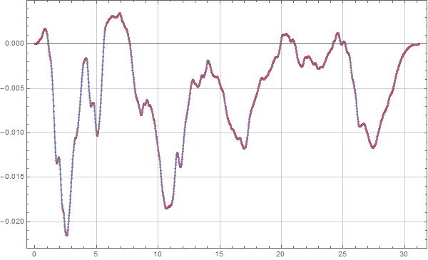
Importing the curve into DPLOT and integrating twice to generate the displacement curve, from which drift was removed. Comparing the exported data,

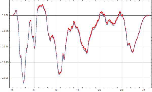
The red line represents DPLOT result, and the blue line is our calculation. These discrepancies are not due to calculation errors but to our use of a cubic function for baseline correction. A linear correction made the results nearly identical, demonstrating that DPLOT Remove Trend function uses a linear adjustment.

Conclusion

This analysis, spanning a day, interspersed with my GRE reading preparation. But it is critical to find the advantage of substituting differential solution approaches for integration in seismic wave analysis. The reference can be found here: LINK1, LINK2, LINK3.

The full script can be downloaded here: DOWNLOAD